
티스토리 뷰
5.1 배경
합성곱 신경망(Convolutional Neural Network)
: 국소적인 영역을 보고 단순 패턴에 자극받는 세포 + 넓은 영역을 보고 복잡 패턴에 자극받는 세포가 계층(layer)를 이룸
5.2 합성곱 연산
1) 합성곱 연산(Convolution)
(1) Convolution
: 하나의 함수가 다른 함수와 얼마나 일치하는지 계산 (하나의 필터를 이동시키며 이미지의 부분들이 필터와 얼마나 일치하는지)
- 하나의 결과값이 생성될 때 입력값 전체가 들어가지 않고 필터가 지나가는 부분만 연산에 포함됨
- 하나의 이미지에 같은 필터를 연달아 적용하므로 가중치가 공유되어 학습 대상이 되는 변수가 적음
- 비선형성 추가 위해 활성화 함수
- Activation map (Feature map) : 필터 하나당 입력 이미지 전체에 대한 필터의 일치 정도
입력이미지의 크기 = I, 필터 크기 = K, 스트라이드 = S, 패딩 = P → Feature map 크기 O = floor[ (I-K+2P)/S + 1 ]
(2) Convolution Layer (nn.Conv2d()) Parameter
in_channels : 입력 채널 수
out_channels : 출력 채널 수
kernel_size : 필터(커널) 크기
stride = 1 : 필터 적용 간격
padding = 0 : 입력 데이터를 추가로 둘러싸는 층의 두께
dilation = 1
groups = 1 : 입력을 채널 단위로 몇 개의 분리된 그룹으로 볼 것인지
bias = True : 편차 사용 여부
padding_mode = 'zeros' : 패딩 적용 방식
- Channels
image,label = mnist_train[0]

# view 또는 unsqueeze → 입력값 형태 : [1,1,28,28]로 변경
image = image.view(-1, image.size()[0], image.size()[1], image.size()[2])

# 1개의 채널을 입력으로 받아 3개의 채널이 나오는 컨볼루션 연산 정의
conv_layer = nn.Conv2d(in_channels=1,out_channels=3,kernel_size=1)
output = conv_layer(image)

# 결과값 형태 : [1,3,28,28] = [B,C,H,W]
print(output.size())

# 출력의 각 채널별 이미지
for i in range(output.size()[1]):
    plt.imshow(output[0,i,:,:].data.numpy(),cmap='gray',vmin=-1,vmax=1)
    plt.show()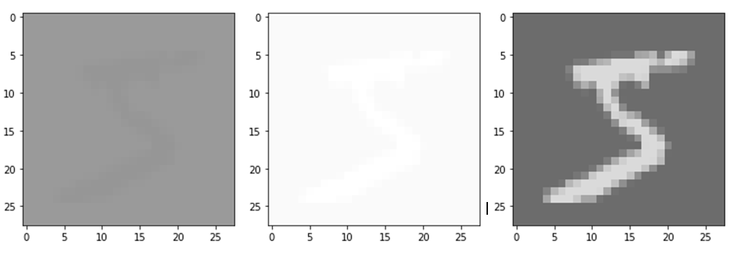
- Kernel Size
conv_layer = nn.Conv2d(in_channels=1,out_channels=1,kernel_size=1)
output = conv_layer(image)
plt.imshow(output[0,0,:,:].data.numpy(),cmap='gray')
plt.show()
print(output.size()) # [1, 1, 28, 28]

conv_layer = nn.Conv2d(in_channels=1,out_channels=1,kernel_size=3)
output = conv_layer(image)
plt.imshow(output[0,0,:,:].data.numpy(),cmap='gray')
plt.show()
print(output.size()) # [1, 1, 26, 26]

conv_layer = nn.Conv2d(in_channels=1,out_channels=1,kernel_size=5)
output = conv_layer(image)
plt.imshow(output[0,0,:,:].data.numpy(),cmap='gray')
plt.show()
print(output.size()) # [1, 1, 24, 24]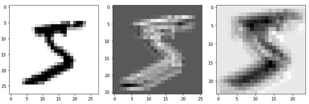
- Stride
conv_layer = nn.Conv2d(in_channels=1,out_channels=1,kernel_size=1,stride=1)
output = conv_layer(image)
plt.imshow(output[0,0,:,:].data.numpy(),cmap='gray')
plt.show()
print(output.size()) # [1, 1, 28, 28]

conv_layer = nn.Conv2d(in_channels=1,out_channels=1,kernel_size=1,stride=3)
output = conv_layer(image)
plt.imshow(output[0,0,:,:].data.numpy(),cmap='gray')
plt.show()
print(output.size()) # [1, 1, 10, 10]

conv_layer = nn.Conv2d(in_channels=1,out_channels=1,kernel_size=1,stride=5)
output = conv_layer(image)
plt.imshow(output[0,0,:,:].data.numpy(),cmap='gray')
plt.show()
print(output.size()) # [1, 1, 6, 6]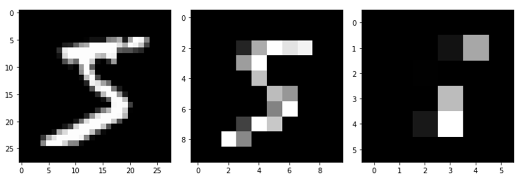
- Padding
conv_layer = nn.Conv2d(in_channels=1,out_channels=1,kernel_size=1,padding=0)
output = conv_layer(image)
plt.imshow(output[0,0,:,:].data.numpy(),cmap='gray')
plt.show()
print(output.size()) # [1, 1, 28, 28]

conv_layer = nn.Conv2d(in_channels=1,out_channels=1,kernel_size=1,padding=1)
output = conv_layer(image)
plt.imshow(output[0,0,:,:].data.numpy(),cmap='gray')
plt.show()
print(output.size()) # [1, 1, 30, 30]

conv_layer = nn.Conv2d(in_channels=1,out_channels=1,kernel_size=1,padding=2)
output = conv_layer(image)
plt.imshow(output[0,0,:,:].data.numpy(),cmap='gray')
plt.show()
print(output.size()) # [1, 1, 32, 32]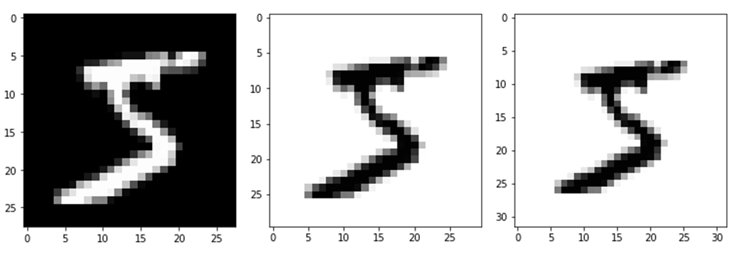
2) CNN(Convolution Neural Network)
(1) CNN : Convolution과 인공신경망 구조가 결합된 형태의 네트워크
- Locality 갖는 모든 신호에서 전체 영역에 대해 서로 동일한 연관성(중요도)으로 처리하는 대신에 특정 범위를 지정해 처리
- Convolution 연산 통해 특징 추출 후, 그 결과값으로 다시 신경망을 돌려 분류
- 학습시켜야 할 가중치 = 필터(커널) 부분 → 특징 더 잘 추출하도록 Parameter update
(2) CNN의 특징
① Locality (Local Connectivity)
- 공간적으로 인접한 신호들에 대한 Correlation 관계를 비선형 필터를 적용해 추출
- 필터를 여러개 적용하면 다양한 Local 특징 추출 가능
- Sub sampling 과정을 거치면서 영상 크기 축소 가능
- Local feature에 대한 filter 연산을 반복적으로 적용하면 점차 Global feature 얻을 수 있음
② Shared Weights
- 동일 계수를 갖는 필터를 영상 전체에 반복 적용 → 변수 # ↓ & Topology Invariance 얻을 수 있음
5.3 Padding, Pooling
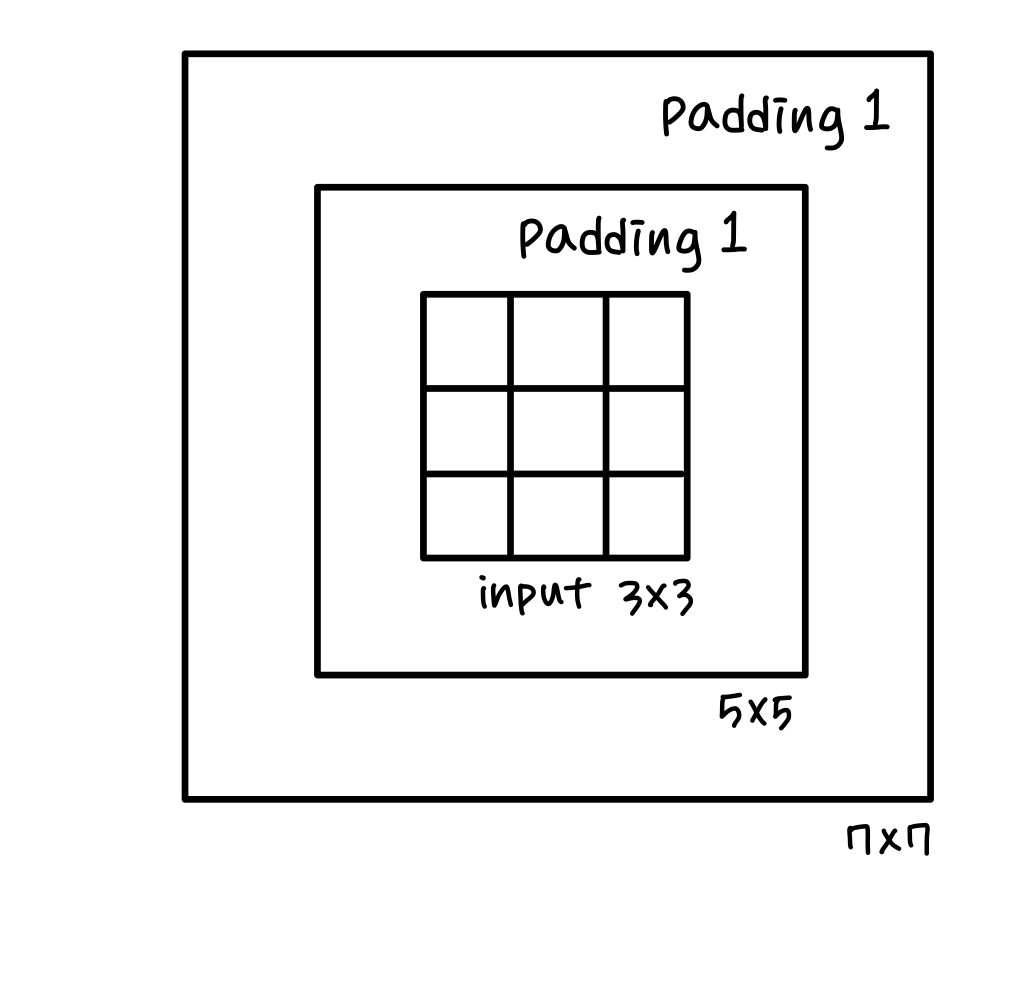
1) 패딩(Padding)
: 입력 이미지에서 충분한 특성을 뽑기 위해 사용
입력이미지의 크기 = I, 필터 크기 = K, 스트라이드 = S, 패딩 = P → Feature map 크기 O = floor[ (I-K+2P)/S + 1 ]
2) 풀링(Pooling)
Downsampling(Subsampling)의 일종, 전체 크기를 줄여줌
(1) Max Pooling
: 일정 크기의 구간 내에서 가장 큰 값만 전달하고 다른 정보는 버리는 방법
= 일정 구간에서 해당 필터의 모양과 가장 비슷한 부분을 전달하는 연산법
(2) Average Pooling
: 일정 크기의 구간 내의 값들의 평균을 전달하는 방법
= 해당 필터의 모양과 평균적으로 얼마나 일치하는지를 뽑아내는 연산법
5.5 Softmax function
1) One-hot encoding
: 본래의 정답을 확률분포로 변환해주는 것 (정답에 해당하는 확률만 1, 나머지는 0)
2) Softmax function
: 신경망의 결과값을 확률로 변경해주는 함수
3) Cross Entropy : Classification task에서 주로 사용하는 Loss function
(1) Entropy
: 불확실성에 대한 정보를 나타내는 척도 = 정보량의 기댓값
H(p) = - ∑ p(x) * logp(x)
p(x) : 일어날 확률, logp(x) : 정보량
일어날 확률이 작을수록 가지고 있는 정보가 크고, 일어날 확률이 클수록 정보가 작음
(2) KL Divergence
: Distribution의 차이를 나타내는 척도 = 비효율적인 정도, D_KL = CE - E
D_KL(p || q) : p를 기준으로 q가 얼마나 다른지 측정 = relative entropy from q to p
(3) Cross Entropy
: 목표로 하는 최적의 확률분포 p와 이를 근사하려는 확률분포 q가 얼마나 다른지 측정
= 원래 p였던 분포를 q로 표현했을 때 드는 비용 측정
= True label(p)과 얼마나 차이 정량화 (목표 : 줄이자)
H(p, q) = - ∑ p(x) * logq(x)
= H(p) + ∑ p(x) * log[p(x)/q(x)]
= H(p) + D_KL(p || q)
의의 : Loss 줄이기 위해 Gradient 구해서 Backprop 하는데,
model output만 변화하고 ∑ p(x)logp(x)는 fixed.
→ Gradient 구할 때 (미분) fixed 부분은 필요 X
→ D_KL 에서 fixed E 부분 빼고 CE만 계산해서 Loss 구함
∴ 교차 엔트로피(CE) 최소화 = KLD 최소화 (H(p)는 fixed 값) → q가 p의 분포와 최대한 같아지도록 하는 것
5.6 모델 구현, 학습 및 결과
1) Setting
import torch
import torch.nn as nn
import torch.optim as optim
import torch.nn.init as init
import torchvision.datasets as dset
import torchvision.transforms as transforms
from torch.utils.data import DataLoader

batch_size = 256
learning_rate = 0.0002
num_epoch = 10

mnist_train = dset.MNIST(root="../", train=True, transform=transforms.ToTensor(), target_transform=None, download=True)
mnist_test = dset.MNIST(root="../", train=False, transform=transforms.ToTensor(), target_transform=None, download=True)

train_loader = DataLoader(mnist_train,batch_size=batch_size, shuffle=True,num_workers=2,drop_last=True)
test_loader = DataLoader(mnist_test,batch_size=batch_size, shuffle=False,num_workers=2,drop_last=True)
(1) Library
torchvision.datasets : 데이터를 읽어오는 모듈
torchvision.transforms : 불러온 이미지를 필요에 따라 변환하는 모듈
torch.utils.data - DataLoader : 데이터를 배치 사이즈로 묶어서 모델에 전달하거나 특정 규칙에 따라 정렬, 섞음으로써 효율적인 학습이 가능하게 하는 모듈
(2) Hyperparameter
: 학습의 대상이 아닌, 학습 이전에 정해놓는 변수
ex. batch_size, learning_rate, num_epoch 등
(3) Data Download & DataLoader
batch_size : dset.MNIST로 정리된 데이터를 batch_size 만큼 묶음
shuffle : 데이터를 섞음
num_workers : 데이터를 묶을 때 사용할 프로세스 개수
drop_last : 묶고 남은 데이터 버릴지 여부
2) CNN 모델 구조
class CNN(nn.Module):
    def __init__(self):
        super(CNN,self).__init__()
        self.layer = nn.Sequential(
            nn.Conv2d(in_channels=1,out_channels=16,kernel_size=5),       # [B,1,28,28] -> [B,16,24,24]
            nn.ReLU(),
            nn.Conv2d(in_channels=16,out_channels=32,kernel_size=5),      # [B,16,24,24] -> [B,32,20,20]
            nn.ReLU(),
            nn.MaxPool2d(kernel_size=2,stride=2),                         # [B,32,20,20] -> [B,32,10,10]
            nn.Conv2d(in_channels=32, out_channels=64, kernel_size=5),    # [B,32,10,10] -> [B,64,6,6]
            nn.ReLU(),
            nn.MaxPool2d(kernel_size=2,stride=2)                          # [B,64,6,6] -> [B,64,3,3]
        )
        self.fc_layer = nn.Sequential(
            nn.Linear(64*3*3,100),                                        # [B,64*3*3] -> [B,100]
            nn.ReLU(),
            nn.Linear(100,10)                                             # [B,100] -> [B,10]
        )

    def forward(self,x):
        out = self.layer(x)                                 # self.layer의 Sequential 연산 차례로 실행
        out = out.view(batch_size,-1)                       # 텐서의 형태를 [batch_size,나머지]로 변경
        out = self.fc_layer(out)
        return out
(1) __init__(self)
- super(CNN, self).__init__() : CNN class의 parent class인 nn.Module 초기화하는 class
- nn.Conv2d()의 H, W 크기 : Feature map 크기 O = floor[ (I-K+2P)/S + 1 ]
- nn.ReLU() : 활성화 함수
- nn.MaxPool2d(kernel_size, stride=None, padding=0, dilation = 1, ...)
- >> kernel_size 영역에서 풀링하고 stride 만큼 이동 → O = floor[ (I-K+2P)/S + 1 ]
- nn.Linear(in_features, out_features) : 분류하고자 하는 Class 수로 뉴런 수 줄여나감
(2) forward(self, x) : self.layer에 정의한 Sequential 연산을 차례로 실행
- .view(batch_size, -1) : 합성곱 연산 텐서 형태를 Linear 연산 텐서 형태인 [batch_size, 나머지]로 변경
3) 손실함수, 최적화함수
device = torch.device("cuda:0" if torch.cuda.is_available() else "cpu")
model = CNN().to(device)

loss_func = nn.CrossEntropyLoss()
optimizer = torch.optim.Adam(model.parameters(), lr=learning_rate)
4) Train 및 손실 시각화
loss_arr =[]
for i in range(num_epoch):
for j,[image,label] in enumerate(train_loader):
x = image.to(device)
y_= label.to(device)
optimizer.zero_grad()
output = model.forward(x)
loss = loss_func(output,y_)
loss.backward()
optimizer.step()
if j % 1000 == 0:
print(loss)
loss_arr.append(loss.cpu().detach().numpy())
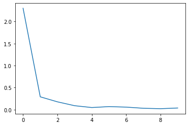
# 학습시 손실 시각화
plt.plot(loss_arr)
plt.show()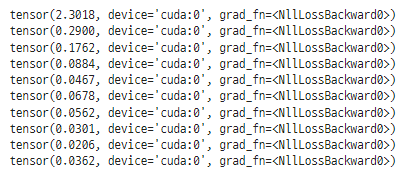
5) Test
correct = 0
total = 0

# Inference Mode
with torch.no_grad():
    for image,label in test_loader:

        x = image.to(device)
        y_= label.to(device)

        output = model.forward(x)
        _,output_index = torch.max(output,1)
        total += label.size(0) # label.size(0) = batch_size
        correct += (output_index == y_).sum().float()

    print("Accuracy of Test Data: {}%".format(100*correct/total))
5.7 주요 모델
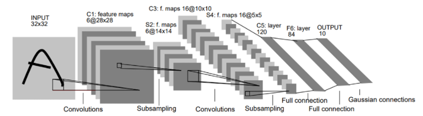
1) LeNet-5
📄Gradient-Based Learning Applied to Document Recognition (MNIST dataset 32x32x1) / Yann LeCun / 1998
- CNN의 기본 구조 갖춤 : 6 layers = 3 Conv(5x5, s=1) + 2 Subsampling(2x2, s=2) + 1 FC
class LeNet(nn.Module):
    def __init__(self):
        super(LeNet, self).__init__()
        self.conv1 = nn.Conv2d(1, 6, kernel_size = 5)      # C1 : O = (32-5+0)/1 + 1 = 28  -> avgpool 14
        self.conv2 = nn.Conv2d(6, 16, kernel_size = 5)     # C3 : O = (14-5+0)/1 + 1 = 10 -> avgpool 5
        self.conv3 = nn.Conv2d(16, 120, kernel_size = 5)   # C5 : O = (5-5+0)/1 + 1 = 1
        self.fc1 = nn.Linear(1*1*120, 84)                  # 1x1 120개의 feature map을 크기 84인 fc에 연결
        self.fc2 = nn.Linear(84, 10)                       # Output : 10개 class (MNIST)

    def forward(self, x):
        x = F.avg_pool2d(torch.tanh(self.conv1(x)), 2) # Conv > Act > Pool
        x = F.avg_pool2d(torch.tanh(self.conv2(x)), 2) # Conv > Act > Pool
        x = torch.tanh(self.conv3(x)) # Conv > Act
        x = x.view(-1, 1*1*120) # 120: fc 처리하기 직전 featuremap 개수 -> flatten
        x = torch.tanh(self.fc1(x)) # FC > Act
        x = self.fc2(x) # FC
        return F.log_softmax(x, dim=1) # Softmax prob
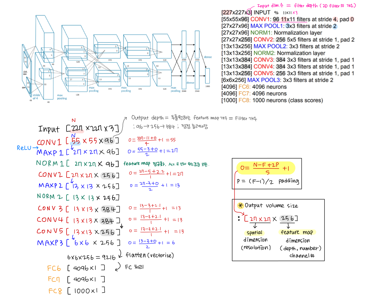
2) AlexNet
- ILSVRC'12 (16.4%). First CNN-based winner → triggered deep learning revolution
- 8 layers (5 Conv + 3 FC), ReLUs, 3 MaxPooling, 2 Norm, Dropout, Data augmentation, 2GPUs 병렬연산
- 점점 Spatial Resolution(Dimension)↓, Feature Channels #↑ .. 추출할 feature의 해상도 낮추면서 개수 늘림(basic)
- smaller compute, still heavy memory, lower accuracy (초기 model이라서)
- Trainable Parameter # 너무 많음 (특히 11x11 conv)
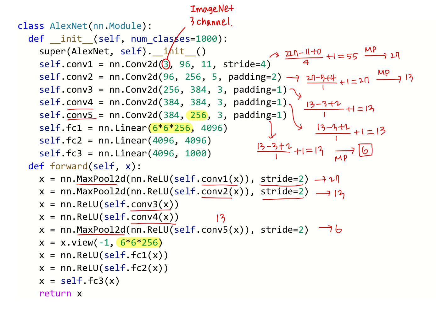
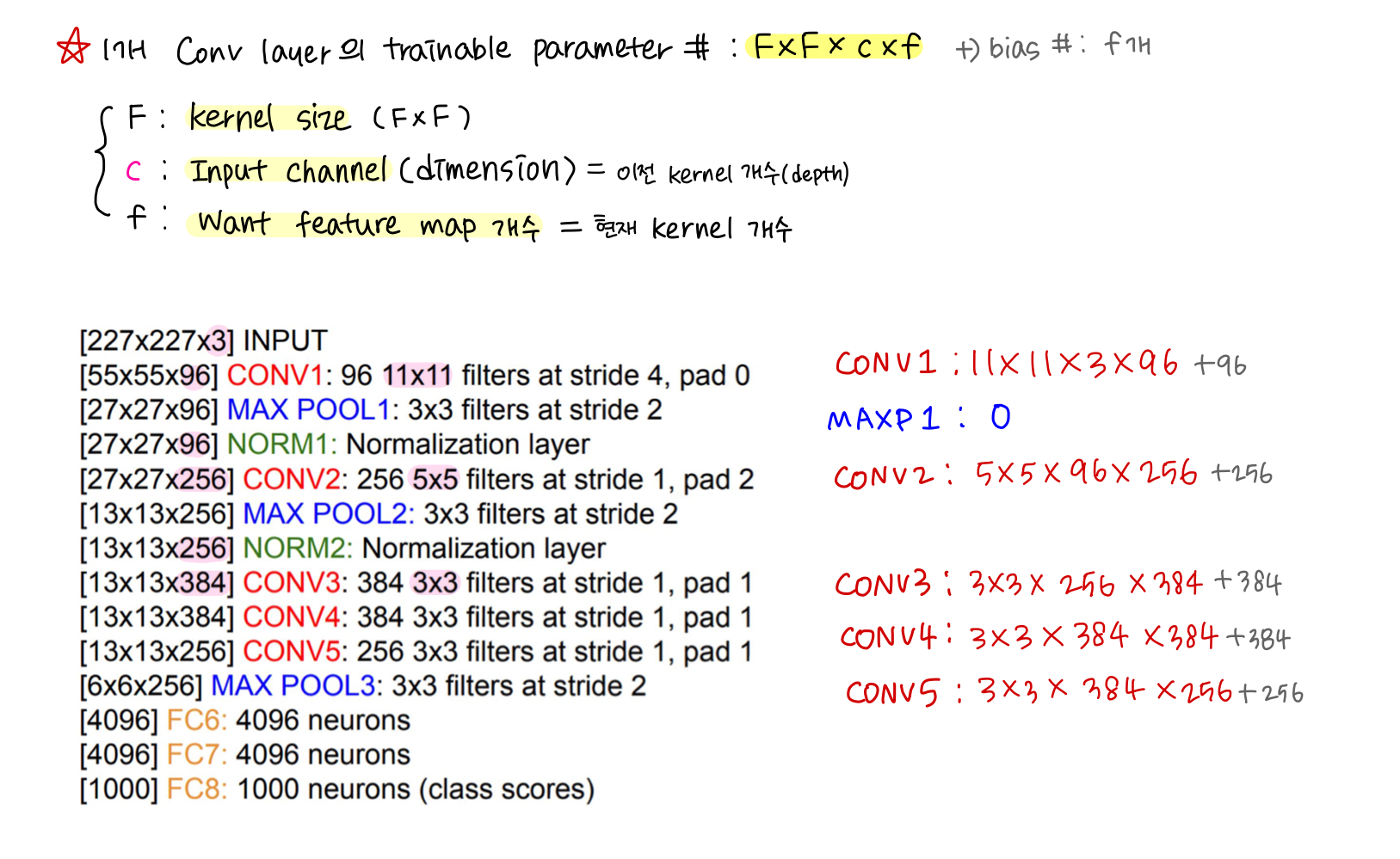
class AlexNet(nn.Module):
  def __init__(self, num_classes=1000):
    super(AlexNet, self).__init__()
    self.conv1 = nn.Conv2d(3, 96, 11, stride=4)
    self.conv2 = nn.Conv2d(96, 256, 5, padding=2)
    self.conv3 = nn.Conv2d(256, 384, 3, padding=1)
    self.conv4 = nn.Conv2d(384, 384, 3, padding=1)
    self.conv5 = nn.Conv2d(384, 256, 3, padding=1)
    self.fc1 = nn.Linear(6*6*256, 4096)
    self.fc2 = nn.Linear(4096, 4096)
    self.fc3 = nn.Linear(4096, 1000)

  def forward(self, x):
    x = nn.MaxPool2d(nn.ReLU(self.conv1(x)), stride=2)
    x = nn.MaxPool2d(nn.ReLU(self.conv2(x)), stride=2)
    x = nn.ReLU(self.conv3(x))
    x = nn.ReLU(self.conv4(x))
    x = nn.MaxPool2d(nn.ReLU(self.conv5(x)), stride=2)
    x = x.view(-1, 6*6*256)
    x = nn.ReLU(self.fc1(x))
    x = nn.ReLU(self.fc2(x))
    x = self.fc3(x)
    return x
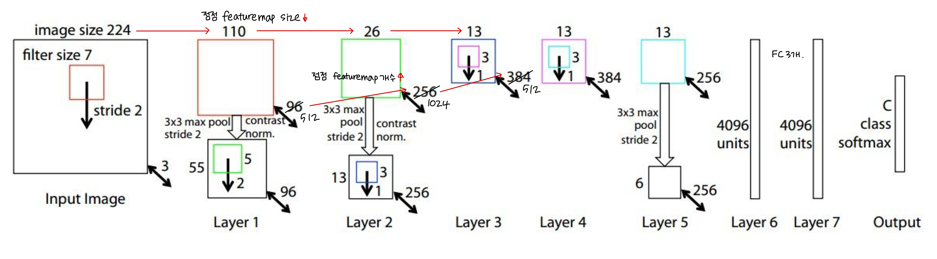
3) ZFNet
📄Visualizing and understanding convolutional networks / Zeiler and Fergus / 2013
- ILSVRC'13 (11.7%). Improved Hyperparameters over AlexNet (8 layers# 같고, 구조 비슷)
- CNN의 Visualizing에 관한 연구
- 네트워크 뒤쪽 conv filter은 앞쪽 filter 보다 complex한 특징 추출하도록 학습됨
- Max Unpooling 개념 제안 : Max 값을 취한 곳의 위치를 기억했다가 unpooling 시 그 위치에 값을 입력
| AlexNet | ZFNet | Change | |
| CONV1 | 11x11, S=4 | 7x7, S=2 | Kernel Size↑ |
| CONV3, 4, 5 | 384, 384, 256 | 512, 1024, 512 | Kernel # ↓ |
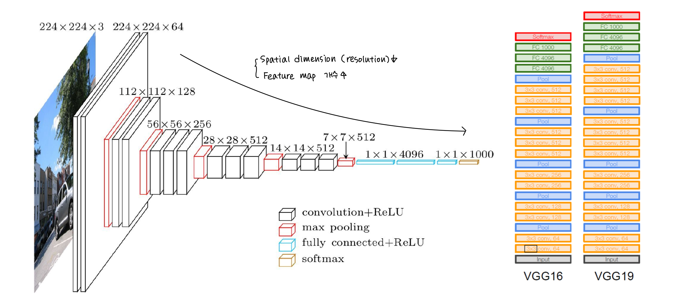
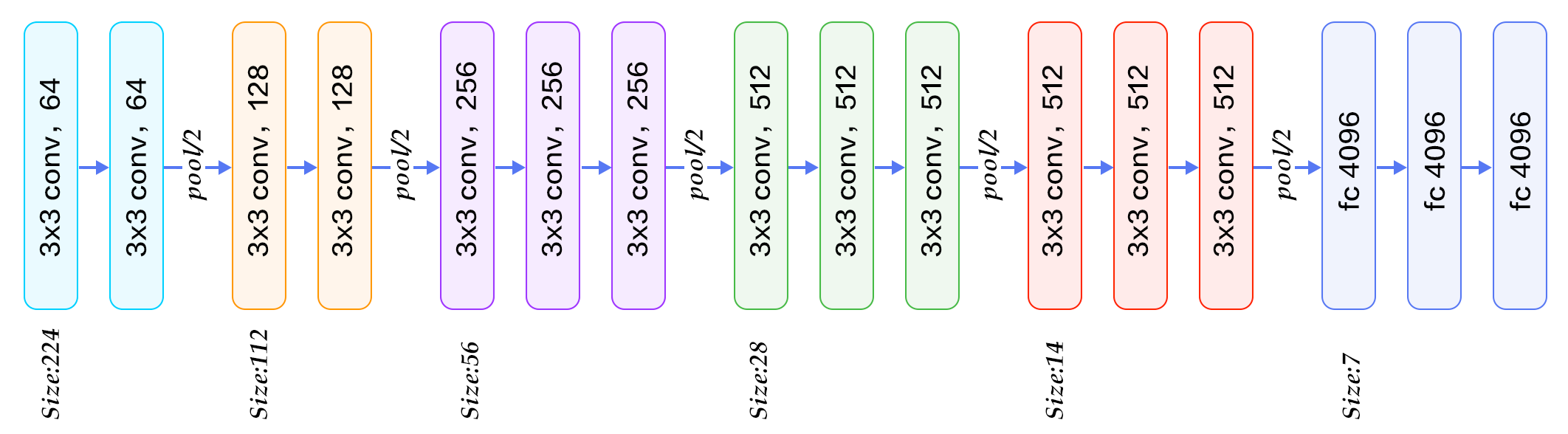
4) VGGNet
📄Very Deep Convolutional Networks For Large-Scale Image Recognition / Simonyan and Andrew / 2014
- 2nd ILSVRC'14 (7.3%)
- 11, 13, 16, 19 layers
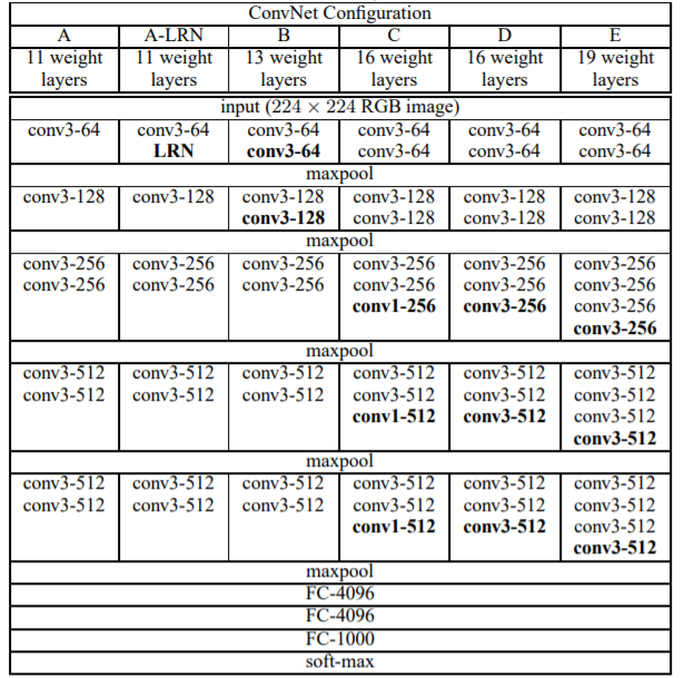
- Small filters, Deeper networks!
- Simple : Only 3x3 Conv(S=1, P=1) + 2x2 MaxPool(S=2) + FC layer
- Highest memory (155M params↑), Most operations(연산량↑) ... 3x3 쓰지만 FC 때문
Why Small filter (3x3)❓
① Stack of three 3x3 Conv(S=1, P=1) : Same Effective Receptive field as one 7x7 Conv
Input data에서 멀리 떨어져 있는 정보가 Conv 거치면서 이웃 pixel로 정보 연쇄적 이동
→ layer 깊어질수록 사용되는 이웃 pixel 정보 많아짐 (Receptive field 증가) & Local + Global 정보 모두 사용 가능
② Fewer parameters → More layers (Deeper) → More ReLUs → More Nonlinearities
3x(3x3xC^2) < 7x7xC^2 (3x3+R)x3 > 7x7+R
(1) 직관적 Code (VGG16 model)
# Basic Blocks
def conv_2_block(in_dim,out_dim):
    model = nn.Sequential(
        nn.Conv2d(in_dim,out_dim,kernel_size=3,padding=1),
        nn.ReLU(),
        nn.Conv2d(out_dim,out_dim,kernel_size=3,padding=1),
        nn.ReLU(),
        nn.MaxPool2d(2,2)
    )
    return model

def conv_3_block(in_dim,out_dim):
    model = nn.Sequential(
        nn.Conv2d(in_dim,out_dim,kernel_size=3,padding=1),
        nn.ReLU(),
        nn.Conv2d(out_dim,out_dim,kernel_size=3,padding=1),
        nn.ReLU(),
        nn.Conv2d(out_dim,out_dim,kernel_size=3,padding=1),
        nn.ReLU(),
        nn.MaxPool2d(2,2)
    )
    return model

# VGG Model
class VGG(nn.Module):
    def __init__(self, base_dim, num_classes=2):
        super(VGG, self).__init__()
        self.feature = nn.Sequential(
            conv_2_block(3,base_dim),
            conv_2_block(base_dim,2*base_dim),
            conv_3_block(2*base_dim,4*base_dim),
            conv_3_block(4*base_dim,8*base_dim),
            conv_3_block(8*base_dim,8*base_dim),
        )
        self.fc_layer = nn.Sequential(
            nn.Linear(8*base_dim * 7 * 7, 100),
            nn.ReLU(True),
            nn.Linear(100, 20),
            nn.ReLU(True),
            #nn.Dropout(),
            nn.Linear(20, num_classes),
        )

    def forward(self, x):
        x = self.feature(x)
        x = x.view(x.size(0), -1)
        x = self.fc_layer(x)
        return x

# Loss function and Optimizer
device = torch.device("cuda:0" if torch.cuda.is_available() else "cpu")
model = VGG(base_dim=16).to(device)
loss_func = nn.CrossEntropyLoss()
optimizer = torch.optim.Adam(model.parameters(), lr=learning_rate)

# Train
for i in range(num_epoch):
    for j,[image,label] in enumerate(train_loader):
        x = image.to(device)
        y_= label.to(device)

        optimizer.zero_grad()
        output = model.forward(x)
        loss = loss_func(output,y_)
        loss.backward()
        optimizer.step()

    if i % 10 ==0:
        print(loss)
(2) 효율적 Code (All VGG models)
class VGG(nn.Module):
    def __init__(self, features, num_classes=1000, init_weights=True, dropout=0.5):
        super(VGG, self).__init__()
        self.features = features
        self.avgpool = nn.AdaptiveAvgPool2d((7, 7))
        self.classifier = nn.Sequential(
            nn.Linear(512 * 7 * 7, 4096),
            nn.ReLU(True),
            nn.Dropout(p=dropout),
            nn.Linear(4096, 4096),
            nn.ReLU(True),
            nn.Dropout(p=dropout),
            nn.Linear(4096, num_classes),
        )
        if init_weights:
            self._initialize_weights()

    def forward(self, x: torch.Tensor) -> torch.Tensor:
        x = self.features(x)
        x = self.avgpool(x)
        x = torch.flatten(x, 1) # x.view(x.size(0),-1)
        x = self.classifier(x)
        return x

    def _initialize_weights(self):
        for m in self.modules():
            if isinstance(m, nn.Conv2d):
                nn.init.kaiming_normal_(m.weight, mode="fan_out", nonlinearity="relu")
                if m.bias is not None:
                    nn.init.constant_(m.bias, 0)
            elif isinstance(m, nn.BatchNorm2d):
                nn.init.constant_(m.weight, 1)
                nn.init.constant_(m.bias, 0)
            elif isinstance(m, nn.Linear):
                nn.init.normal_(m.weight, 0, 0.01)
                nn.init.constant_(m.bias, 0)


def make_layers(cfg, batch_norm=False):
    layers = []
    in_channels = 3
    for v in cfg:
        if v == "M":
            layers += [nn.MaxPool2d(kernel_size=2, stride=2)]
        else:
            v = cast(int, v)
            conv2d = nn.Conv2d(in_channels, v, kernel_size=3, padding=1)
            if batch_norm:
                layers += [conv2d, nn.BatchNorm2d(v), nn.ReLU(inplace=True)]
            else:
                layers += [conv2d, nn.ReLU(inplace=True)]
            in_channels = v
    return nn.Sequential(*layers)


cfgs = {
    "A": [64, "M", 128, "M", 256, 256, "M", 512, 512, "M", 512, 512, "M"],
    "B": [64, 64, "M", 128, 128, "M", 256, 256, "M", 512, 512, "M", 512, 512, "M"],
    "D": [64, 64, "M", 128, 128, "M", 256, 256, 256, "M", 512, 512, 512, "M", 512, 512, 512, "M"],
    "E": [64, 64, "M", 128, 128, "M", 256, 256, 256, 256, "M", 512, 512, 512, 512, "M", 512, 512, 512, 512, "M"],
}
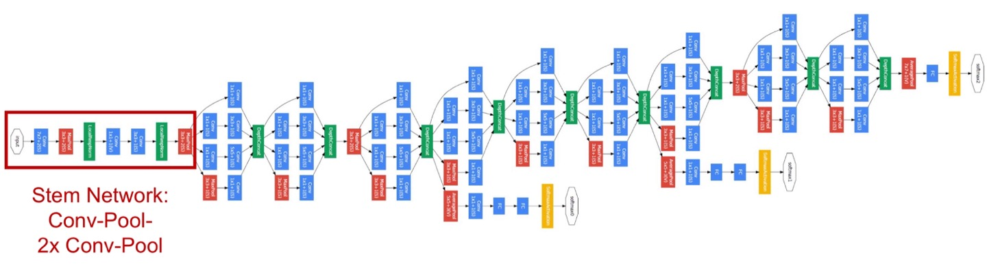
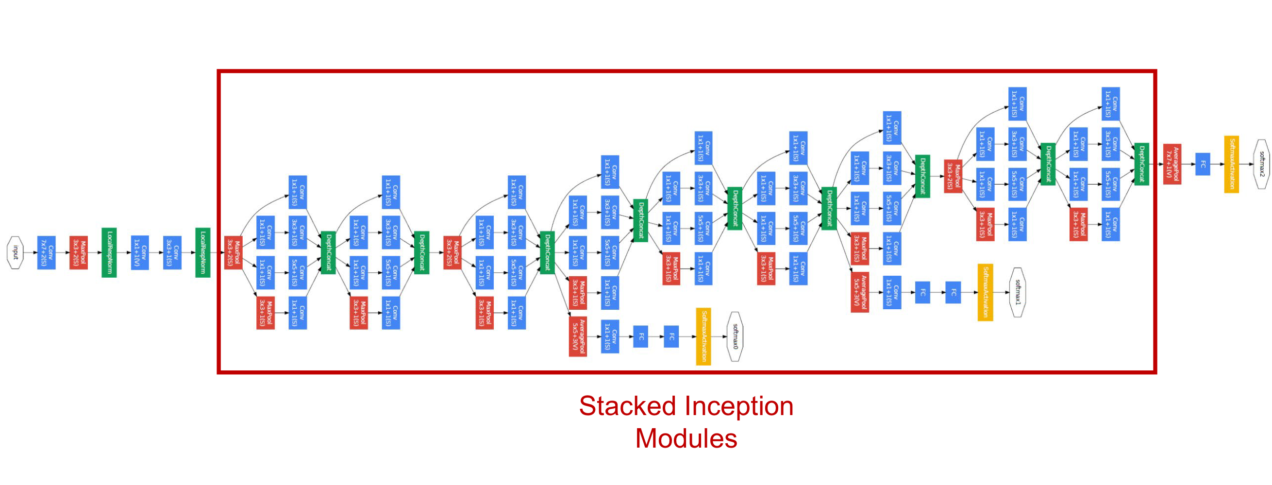
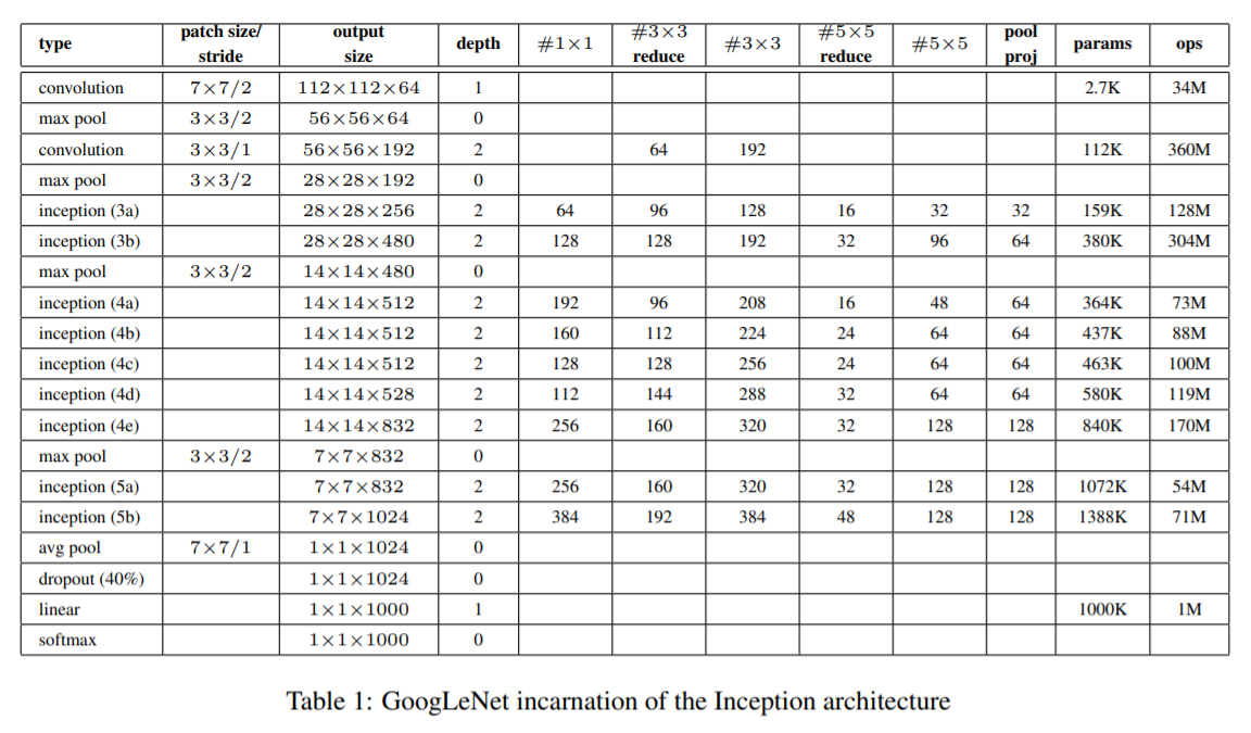
5) GoogLeNet
📄Going deeper with convolutions / Szegedy / 2015
- 1st ILSVRC'14 (6.7%). 22 layers (deeper networks)
- Deeper networks, with Computational efficiency! (Parameter↓)
- Most efficient (Only 5 million params)
- Complicated
(1) Stem Network (conv-pool-conv-conv-pool)
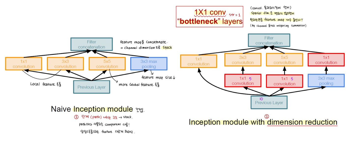
(2) Stacked Inception module (Block 단위) : Computational efficiency↑
① Path 4개 나뉘는 구조 : good Local network topology (network within a network)
: Varying filter size conv/pool operations (1x1, 3x3, 5x5 conv, 3x3 maxpool) = path 마다 사용되는 component 달라서
다양한 feature 추출 가능 → feature maps를 concate 해서 채널 차원으로 stack
② 1x1 Conv Bottleneck layers
: Spatial Dimension은 유지하면서, 원하는만큼 Feature map Dimension 줄이는 것 (Parameter↓)
각각의 연산 결과들을 채널 차원으로 concate ← S=1, P을 조정하여 O = N 유지 (H,W의 resolution 같아야 함) *code
③ Multiple intermediate classification heads (Auxiliary Classifier, 보조 분류기) - 학습 과정에서만 사용 (test X)
: 학습 시, 모델 output을 앞부분에서도 중간중간 꺼내서 추가적인 gradient 전달 → Vanishing gradient 문제 해결
모델이 깊어지면서 마지막 단의 Classifier에서 발생한 Loss가 모델 입력 부분까지 전달 안 되는 현상 극복 (학습 보조)
def conv_1(in_dim,out_dim):
    model = nn.Sequential(
        nn.Conv2d(in_dim,out_dim,1,1),
        nn.ReLU(),
    )
    return model

def conv_1_3(in_dim,mid_dim,out_dim):
    model = nn.Sequential(
        nn.Conv2d(in_dim,mid_dim,1,1),
        nn.ReLU(),
        nn.Conv2d(mid_dim,out_dim,3,1,1),
        nn.ReLU()
    )
    return model

def conv_1_5(in_dim,mid_dim,out_dim):
    model = nn.Sequential(
        nn.Conv2d(in_dim,mid_dim,1,1),
        nn.ReLU(),
        nn.Conv2d(mid_dim,out_dim,5,1,2),
        nn.ReLU()
    )
    return model

def max_3_1(in_dim,out_dim):
    model = nn.Sequential(
        nn.MaxPool2d(3,1,1),
        nn.Conv2d(in_dim,out_dim,1,1),
        nn.ReLU(),
    )
    return model

class inception_module(nn.Module):
    def __init__(self,in_dim,out_dim_1,mid_dim_3,out_dim_3,mid_dim_5,out_dim_5,pool):
        super(inception_module,self).__init__()
        self.conv_1 = conv_1(in_dim,out_dim_1)
        self.conv_1_3 = conv_1_3(in_dim,mid_dim_3,out_dim_3)
        self.conv_1_5 = conv_1_5(in_dim,mid_dim_5,out_dim_5)
        self.max_3_1 = max_3_1(in_dim,pool)

    def forward(self,x):
        out_1 = self.conv_1(x)
        out_2 = self.conv_1_3(x)
        out_3 = self.conv_1_5(x)
        out_4 = self.max_3_1(x)
        output = torch.cat([out_1,out_2,out_3,out_4],1)
        return output


class GoogLeNet(nn.Module):
    def __init__(self, base_dim, num_classes=2):
        super(GoogLeNet, self).__init__()
        self.num_classes=num_classes
        self.layer_1 = nn.Sequential(
            nn.Conv2d(3,base_dim,7,2,3),
            nn.MaxPool2d(3,2,1),
            nn.Conv2d(base_dim,base_dim*3,3,1,1),
            nn.MaxPool2d(3,2,1),
        )
        self.layer_2 = nn.Sequential(
            inception_module(base_dim*3,64,96,128,16,32,32),
            inception_module(base_dim*4,128,128,192,32,96,64),
            nn.MaxPool2d(3,2,1),
        )
        self.layer_3 = nn.Sequential(
            inception_module(480,192,96,208,16,48,64),
            inception_module(512,160,112,224,24,64,64),
            inception_module(512,128,128,256,24,64,64),
            inception_module(512,112,144,288,32,64,64),
            inception_module(528,256,160,320,32,128,128),
            nn.MaxPool2d(3,2,1),
        )
        self.layer_4 = nn.Sequential(
            inception_module(832,256,160,320,32,128,128),
            inception_module(832,384,192,384,48,128,128),
            nn.AvgPool2d(7,1),
        )
        self.layer_5 = nn.Dropout2d(0.4)
        self.fc_layer = nn.Linear(1024,self.num_classes)


    def forward(self, x):
        out = self.layer_1(x)
        out = self.layer_2(out)
        out = self.layer_3(out)
        out = self.layer_4(out)
        out = self.layer_5(out)
        out = out.view(batch_size,-1)
        out = self.fc_layer(out)
        return out
# Optimizer & Loss function
device = torch.device("cuda:0" if torch.cuda.is_available() else "cpu")
model = GoogLeNet(base_dim=64).to(device)
loss_func = nn.CrossEntropyLoss()
optimizer = optim.Adam(model.parameters(),lr=learning_rate)
# Train
for i in range(num_epoch):
for j,[image,label] in enumerate(train_loader):
x = image.to(device)
y_= label.to(device)
optimizer.zero_grad()
output = model.forward(x)
loss = loss_func(output,y_)
loss.backward()
optimizer.step()
if i % 10 ==0:
print(loss)
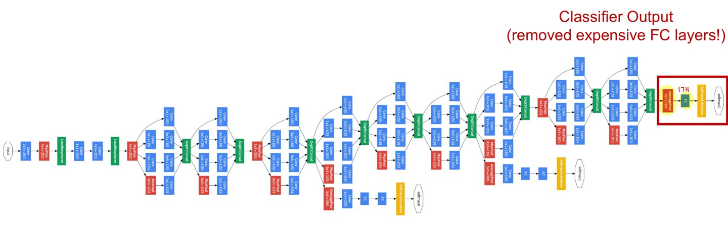
(3) Classifier : GAP (NO FC, only 1 FC) : Channel # 유지하면서, Spatial Dimension 줄이는 것 (Vectorize)
Pooling has No trainable params → Only 5 million params (27x less than VGG16)! (Parameter↓)
6) ResNet
📄Deep residual learning for image recognition / He / 2016
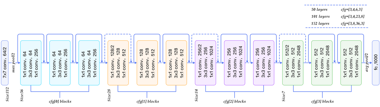
- 1st ILSVRC'15 (3.57%). 152 layers (Revolution of Depths)
- 초기에 size ↓ : 7x7 Conv1 거치고 바로 MaxPooling → Image size (Spatial Dimension) : 56x56 → 유지
- Total Depth of 34, 50, 101, or 152 layers models for ImageNet : Deeper model 성능 best
- Moderate efficiency / depending on model, highest accuracy
Degradation problem❓
: Deeper model(56-layers) 일수록 Training and Test error both ↑
(Training error도 높으므로 Overfitting X, 점점 error 줄어들므로 Vanishing gradient X)
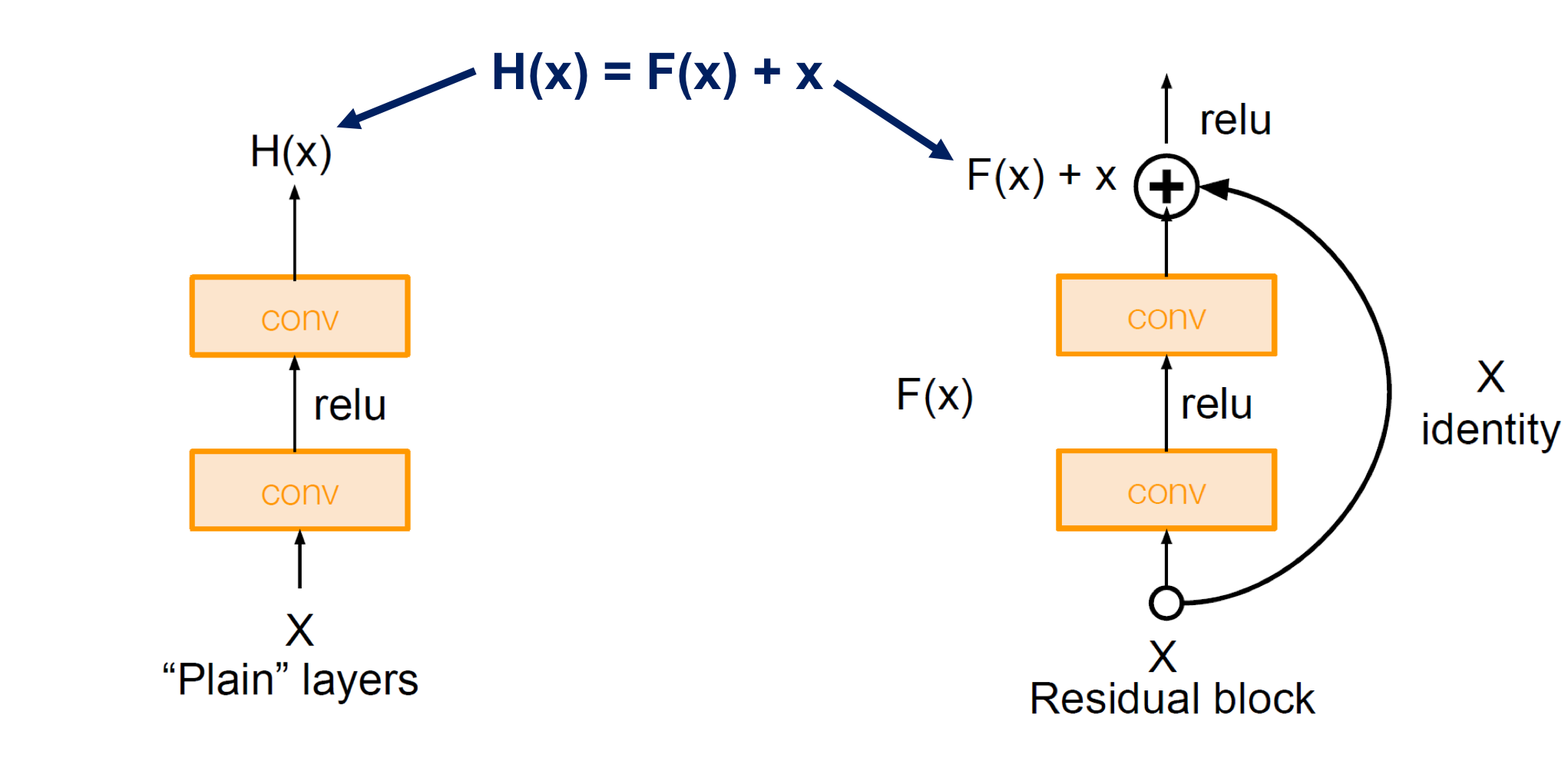
✅ Solution (유일x) : Residual Learning
(1) Stacked Residual blocks F(x) = H(x) - x instead of H(x) directly
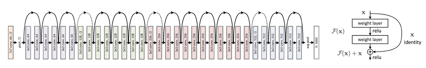
: Skip connection을 통한 Identity mapping → H(x) = F(x) + x ... Every Residual box has two 3x3 Conv
- 특정 위치에 입력 x가 들어왔을 때 conv를 통과한 결과인 F(x)와 입력으로 들어온 결과 x를 더해 다음 layer에 전달
- 이전 단계에서 뽑았던 특성들을 변형시키지 않고 그대로 더해 전달하므로 입력단의 단순 특성 + 출력단의 복잡 특성 모두 사용
- '+' 연산은 backprop할 때 기울기가 1이라 Loss가 줄어들지 않고 모델 앞부분까지 잘 전파됨 (학습시 보조 분류기 필요 X)
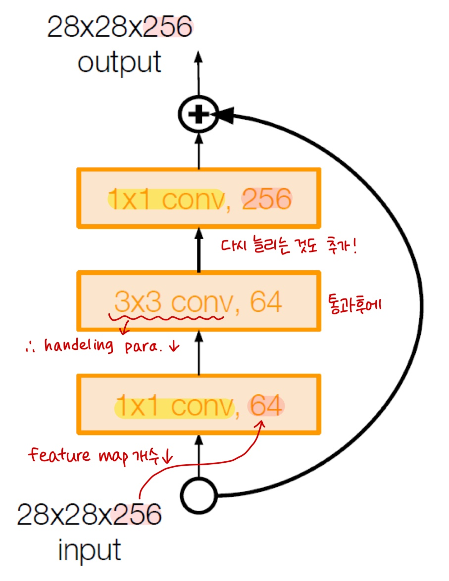
+) 1x1 Conv Bottleneck layers (50+ models)
Improving efficiency for Deeper models (50+) : 깊어질수록 params# 많아지는 문제 극복
28x28x256 Input → 1x1 conv, 64 filters (채널 방향 압축, reduce feature maps) *Stride=2 → 1/2배로 size 압축
→ 3x3 conv handeling only 64 feature maps (압축된 상태에서 원하는 추가 특성 뽑아냄) !
→ 1x1 conv, 256 filters (채널 수 원상태로 늘려줌, project back to 256) → 28x28x256 output
(2) Strided Convolution for Downsampling : Spatial Dimension↓ (Pooling layer 대체)
- 실선 = Spatial Dimension 바뀌지 X 경우
- 점선 = Downsampling으로 인해 Spatial Dimension 바뀌는 경우 *F=1, S=2 → 1/2배로 size 압축
: 이전 단계의 Feature map의 Spatial Dimension 1/2배씩↓ + Feature map # (= Filter #) 2배씩↑
(3) Classifier : GAP (NO FC, only 1 FC) ... only FC1000 to output class
def conv_block_1(in_dim,out_dim,act_fn,stride=1):
    model = nn.Sequential(
        nn.Conv2d(in_dim,out_dim, kernel_size=1, stride=stride),
        act_fn,
    )
    return model


def conv_block_3(in_dim,out_dim,act_fn):
    model = nn.Sequential(
        nn.Conv2d(in_dim,out_dim, kernel_size=3, stride=1, padding=1),
        act_fn,
    )
    return model

class BottleNeck(nn.Module):
    def __init__(self,in_dim,mid_dim,out_dim,act_fn,down=False):
        super(BottleNeck,self).__init__()
        self.down=down

        # Feature map size가 1/2로 줄어드는 경우 (점선)
        if self.down:
            self.layer = nn.Sequential(
              conv_block_1(in_dim,mid_dim,act_fn,2), # Stride=2
              conv_block_3(mid_dim,mid_dim,act_fn),
              conv_block_1(mid_dim,out_dim,act_fn),
            )
            self.downsample = nn.Conv2d(in_dim,out_dim,1,2) # Strided Convolution

        # Feature map size가 그대로인 경우 (실선)
        else:
            self.layer = nn.Sequential(
                conv_block_1(in_dim,mid_dim,act_fn),
                conv_block_3(mid_dim,mid_dim,act_fn),
                conv_block_1(mid_dim,out_dim,act_fn),
            )

        # 더하기를 위해 차원을 맞춰주는 1x1 Convolution -> In/Out channel 같아짐
        self.dim_equalizer = nn.Conv2d(in_dim,out_dim,kernel_size=1)

    def forward(self,x):
        if self.down:
            downsample = self.downsample(x) # Strided Convolution
            out = self.layer(x)             # Feature map size 1/2로 줄어듦
            out = out + downsample
        else:
            out = self.layer(x)
            if x.size() is not out.size():  # In/Out channel 다를 경우
                x = self.dim_equalizer(x)   # 차원 맞춰준 후
            out = out + x                   # 더하기
        return out

# ResNet-50
class ResNet(nn.Module):

    def __init__(self, base_dim, num_classes=2):
        super(ResNet, self).__init__()
        self.act_fn = nn.ReLU()

        self.layer_1 = nn.Sequential(
            nn.Conv2d(3,base_dim,7,2,3),
            nn.ReLU(),
            nn.MaxPool2d(3,2,1),
        )
        self.layer_2 = nn.Sequential(
            BottleNeck(base_dim,base_dim,base_dim*4,self.act_fn),
            BottleNeck(base_dim*4,base_dim,base_dim*4,self.act_fn),
            BottleNeck(base_dim*4,base_dim,base_dim*4,self.act_fn,down=True),
        )
        self.layer_3 = nn.Sequential(
            BottleNeck(base_dim*4,base_dim*2,base_dim*8,self.act_fn),
            BottleNeck(base_dim*8,base_dim*2,base_dim*8,self.act_fn),
            BottleNeck(base_dim*8,base_dim*2,base_dim*8,self.act_fn),
            BottleNeck(base_dim*8,base_dim*2,base_dim*8,self.act_fn,down=True),
        )
        self.layer_4 = nn.Sequential(
            BottleNeck(base_dim*8,base_dim*4,base_dim*16,self.act_fn),
            BottleNeck(base_dim*16,base_dim*4,base_dim*16,self.act_fn),
            BottleNeck(base_dim*16,base_dim*4,base_dim*16,self.act_fn),
            BottleNeck(base_dim*16,base_dim*4,base_dim*16,self.act_fn),
            BottleNeck(base_dim*16,base_dim*4,base_dim*16,self.act_fn),
            BottleNeck(base_dim*16,base_dim*4,base_dim*16,self.act_fn,down=True),
        )
        self.layer_5 = nn.Sequential(
            BottleNeck(base_dim*16,base_dim*8,base_dim*32,self.act_fn),
            BottleNeck(base_dim*32,base_dim*8,base_dim*32,self.act_fn),
            BottleNeck(base_dim*32,base_dim*8,base_dim*32,self.act_fn),
        )
        self.avgpool = nn.AvgPool2d(7,1)
        self.fc_layer = nn.Linear(base_dim*32,num_classes)

    def forward(self, x):
        out = self.layer_1(x)
        out = self.layer_2(out)
        out = self.layer_3(out)
        out = self.layer_4(out)
        out = self.layer_5(out)
        out = self.avgpool(out)
        out = out.view(batch_size,-1)
        out = self.fc_layer(out)

        return out
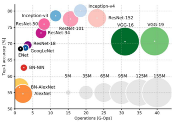
Network Complexity
'DL > Pytorch' 카테고리의 다른 글
| [Ch7] 학습 시 생길 수 있는 문제점 및 해결방안 (0) | 2022.01.22 |
|---|---|
| [Ch6] 순환신경망(RNN) (0) | 2022.01.20 |
| [Ch4] 인공 신경망(ANN) (0) | 2022.01.15 |
| [Ch3] 선형회귀분석 (0) | 2022.01.15 |
| [Ch1, 2] Deep Learning & Pytorch (0) | 2022.01.10 |