티스토리 뷰
7.1 Introduction
Noise : degradation in img signal, caused by external disturbance
Depending on Type of disturbance → Type of errors on output img → Type of noise on img
→ Choose appropriate method(Image Restoration) for reducing each type of noise !
7.2 Types of noise
1) Salt and pepper noise
(1) Salt and pepper noise
= Impulse noise, shot noise, binary noise
- caused by sharped, sudden disturbances
- appeared randomly scattered white and black (or both) pixels over img
(2) imnoise(t, 'salt & papper')
- Optional parameter : the amount of noise (fraction of pixels to be corrupted) = 0~1 (default = 0.1)
>> tw=imread('twins.tif');
>> t=rgb2gray(tw);
>> t_sp=imnoise(t,'salt & pepper', 0.2);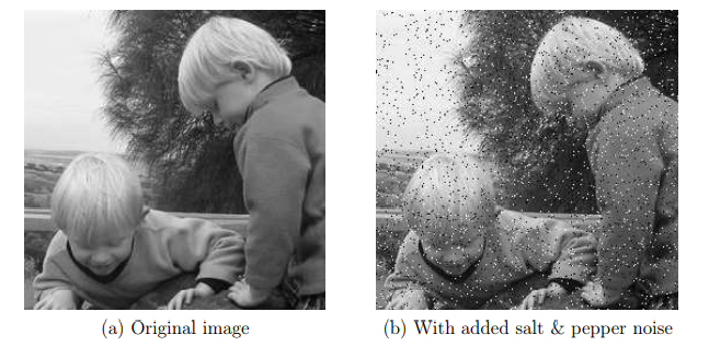
2) Gaussian noise
(1) Gaussian noise
- An idealized form of white noise which is normally distributed
- caused by random fluctuations in the signal
- can be modelled by random values added to an img
Gaussian Noisy img : I + N
I : an image matrix whose elements are pixel values of img
N : a noise matrix whose elements are normally distributed
(2) Implementation by imnoise(t, 'gaussian')
- Optional parameter : mean and variance of noise (defalut = 0 and 0.01)
>> t_ga=imnoise(t,'gaussian');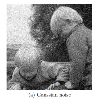
3) Speckle noise
(1) Speckle noise
= multiplicative noise
- major problem in some radar applications
- can be modelled by random values multiplied by pixel value
Speckle Noisy img : I * (1+N)
I : an image matrix whose elements are pixel values of img
N : a noise matrix whose elements are normally distributed
(2) Implementation by imnoise(t, 'speckle')
- Optional parameter : variance of noise N (default = 0.04)
>> t_spk=imnoise(t,'speckle');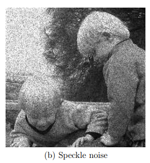
4) Periodic noise
(1) Periodic noise
- Periodic img → img corrupted by periodic noise
- Effect of bars over img
(2) Implementation by hands
- imnoise function (X)
- Easy to create by adding a periodic matrix (using a trigonometric function) to img
>> s=size(t);
>> [x,y]=meshgrid(1:s(1),1:s(2));
>> p=sin(x/3+y/5)+1;
>> t_pn=(im2double(t)+p/2)/2;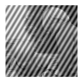
+) How to Clean noise
- Salt & pepper noise, Gaussian noise, Speckle noise can be cleaned by using spatial filtering techniques
- Periodic noise requires img transforms !
7.3 Cleaning salt & pepper noise
1) Low pass filtering
Pixels corrupted by salt & pepper noise : High freq components of img
Loss-pass filter (Average filter) : reducing High freq
>> a3=fspecial('average');
>> t_sp_a3=filter2(a3,t_sp);

>> a7=fspecial('average',[7,7]);
>> t_sp_a7=filter2(a7,t_sp);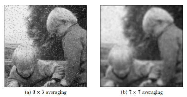
(a) 3x3 : Smeard effect (still noisy)
(b) 7x7 : More smeard with a larger filter
2) Median filtering
(1) Median filtering
Median filtering : Great method for removal of salt & pepper noise
Median filter : a non-linear spatial filter, using 3x3 mask, the output value is median of values in the mask
Median value of a set : middle value when they are sorted (If even number, median is mean of middle two)
Noisy value (very large or very small values) : value at the top or bottom of sorted list
→ Median value will replace a Noisy value with one closer to its surroundings
(2) Implementation by medfilt2 function
>> t_sp_m3=medfilt2(t_sp);
>> t_sp2=imnoise(t,’salt & pepper’,0.2);
>> t_sp2_m3=medfilt2(t_sp2);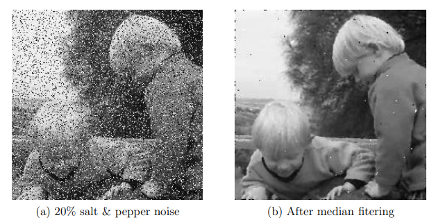
>> t_sp2_m5=medfilt2(t_sp2,[5,5]);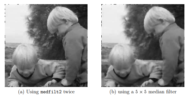
(a) Second application of 3x3 median filter (using medfilt2 twice)
(b) Optional parameter : mask size (using a 5x5 median filter)
3) Rank-order filtering
(1) Rank-order filtering
- Ordering the set and taking the n-th value, for some predetermined value of n
- Median filtering is a special case of Rank-order filtering
Median filtering using 3x3 mask == Rank-order filtering with n=5
Median filtering using 5x5 mask == Rank-order filtering with n=13
(2) Implementation by ordfilt2 function
- To choose the median of non-rectangular masks (Ex. cross shape)
- First element : Noise (Salt & pepper)
- Second element : Value of ordered set
- Thrid element : Domain (the non-zero values of which specify the mask)
>> ordfilt2(t_sp,3,[0 1 0;1 1 1;0 1 0]);
>> ordfilt2(t_sp,5,[0 0 1 0 0;0 0 1 0 0;1 1 1 1 1;0 0 1 0 0;0 0 1 0 0])
4) An outlier method
(1) Why
- Median filtering is slow (each pixel requires the sorting) → To overcome this, Outlier method was proposed
- Outlier method : The use of cleaning salt and papper noise by treating noisy pixels as outlier(pixels whose grey values are significantly different from those of their neighbors)
(2) How
① Choose a threshold value D
② For a given pixel, compare its value p with the mean m of the values of its eight neighbors
③ If | p-m | > D, classify the pixel as noisy, otherwise not
④ If the pixel is noisy, replace its value with m, otherwise leave its value unchanged
(3) Implementation
▪ Produce a matrix r consisting of 1's at only places where difference of the original and filter are greater than D
r : 1's at noisy pixels → (1-r) : 1's at not noisy pixels
r * filter = replacing noisy values(r) with averages(m)
(1-r) * original values = the rest of the output
function res=outlier(im,d)
% OUTLIER(IMAGE,D) removes salt and pepper noise using an outlier method.
% This is done by using the following algorithm:
%
% For each pixel in the image, if the difference between its grey value
% and the average of its eight neighbours is greater than D, it is
% classified as noisy, and its grey value is changed to that of the
% average of its neighbours.
%
% IMAGE can be of type UINT8 or DOUBLE; the output is of type
% UINT8. The threshold value D must be chosen to be between 0 and 1.

f=[0.125 0.125 0.125; 0.125 0 0.125; 0.125 0.125 0.125];
imd=im2double(im);
imf=filter2(f,imd);
r=abs(imd-imf)-d>0;
res=im2uint8(r.*imf+(1-r).*imd);
▪ Not automatic : threshold(D) must be chosen for best results
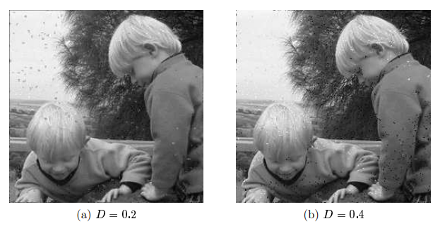
If D is too small , too many 'non-noisy' pixels will be classified as noisy → average → blurring effect
(a) D=0.2 : lower value of D tends to remove noise from dark areas
(+) D=0.3 : mid-way value produces an acceptable result (median filtering보다는 X)
(b) D=0.4 : higher value of D tends to remove noise from light areas
If D is too large, not enough noisy pixels will be classified as noisy → little chanege in the output
▪ Outlier method = Quick and dirty method for cleaning salt & pepper noise when Median filter proves too slow
(Salt & pepper noise 제거 위해서는 Median filter가 더 좋은데, 빨리 끝내야 한다면 Outlier method 사용해라)
7.4 Cleaning Gaussian noise
1) Image Averaging
(1) When
Sometimes many different copies of img corrupted with Gaussian noise (not only 1 img)
- Satellite imaging : Satellite passes over the same spot many times → many different imgs of same place
- Microscopy : many different imgs of the same object
* This method only works if the Gaussian noise has mean 0
(2) How
To simply take the average (the mean) of all the imgs
M : matrix of orignal values
N_i : matrix of normally distributed random noise values with mean 0
M+N_i : i-th noisy img
M' : the mean value of imgs
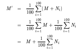
Mean of all the N_i's will be close to zero (The greater the number of N_i's, the closer to zero)
Approximation is closer for larger number of imgs M+N_i

(3) Implementation
① Create 10 different versions with Gaussian noise, and take the average of them
(Empty 3-dimensional array of depth 10, filled each level with a noisy img)
>> s=size(t);
>> t_ga10=zeros(s(1),s(2),10);
>> for i=1:10 t_ga10(:,:,i)=imnoise(t,'gaussian');end
② Take the average
- Optional parameter 3 : taking the mean along the third dimension of array
- (b) Better result is obtained bu taking the average of 100 imgs (depth 100)
>> t_ga10_av=mean(t_ga10,3);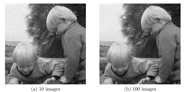
2) Averaging filtering
(1) Trade-off blurring for noise reduction
- If the Gaussian noise has mean 0, average filter would average the noise to zero
(The larger the size of filter mask, the closer to zero)
- BUT, averaging tends to blur an img (trade off)
∴ Some noise reduction BUT smeary(blurring) nature of the resulting imgs
>> a3=fspecial('average');
>> a5=fspecial('average',[5,5]);
>> tg3=filter2(a3,t_ga);
>> tg5=filter2(a5,t_ga);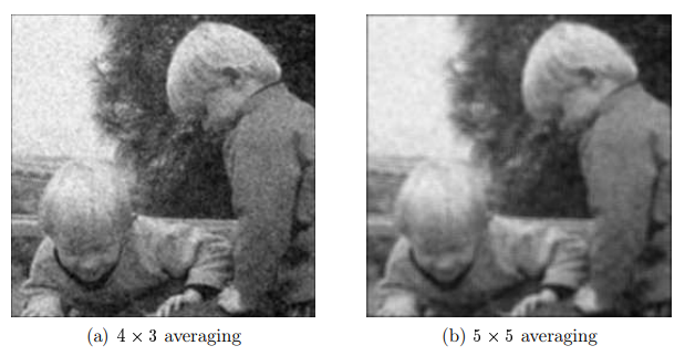
3) Wiener filtering
(1) Wiener filtering
M : Original img
R : Restored version of img
Minimize the least squares of all differences bw R and M

Wiener filtering : non-linear spatial filter ; moving a mask across the noisy img, pixel by pixel
→ Output img = the grey values of whose pixels are based on the values under the mask
(2) Theoretical calculation
N : Noise (normally distributed with mean 0)
M' = M+N : Degraded (Noisy) img
However, within our mask, the mean may not be zero
m_f : mean of mask = mean of all grey values under the mask
σ_f ^2 : variance in the mask = variance of all grey values under the mask
σ_g ^2 : variance of the noise over the entire img
g : current value of the pixel in the noisy img
→ Output value can be calculated as

(3) Implementation by wiener2 function
▪ Slight variant of the above equation for using efficient wiener filtering
n : the computed noise variance (calculated by taking the mean of all values of σ_f ^2 over entire img)

▪ Optional parameter : mask size (default = 3x3)
>> t1=wiener2(t_ga);
>> t2=wiener2(t_ga,[5,5]);
>> t3=wiener2(t_ga,[7,7]);
>> t4=wiener2(t_ga,[9,9]);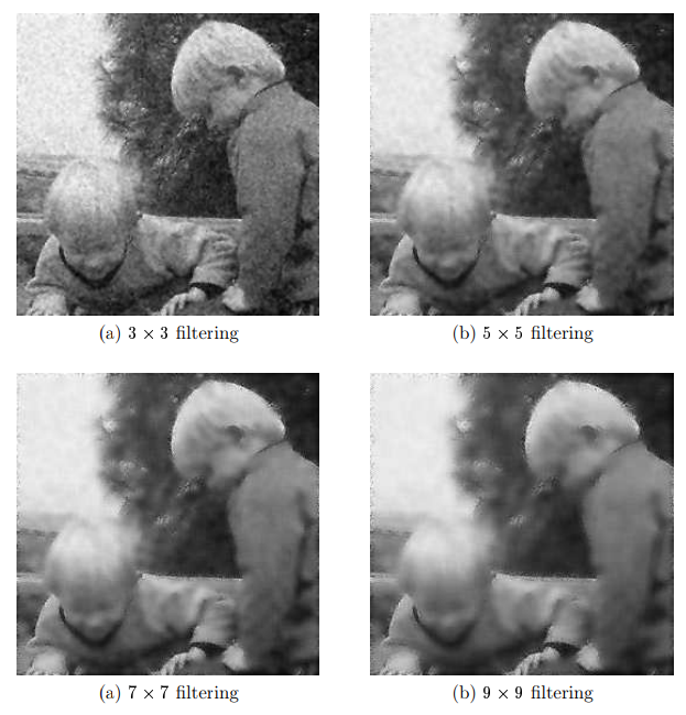
▪ Being a Low-pass filter, Wiener filtering tends to blur edges and high freq of img (better than LPBF)
>> t2=imnoise(t,'gaussian',0,0.005);
>> imshow(t2)
>> t2w=wiener2(t2,[7,7]);
>> figure,imshow(t2w)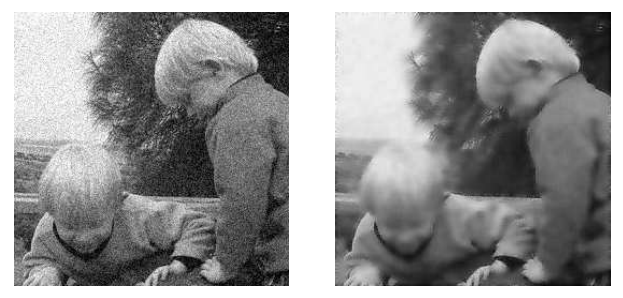
'DIP > Matlab' 카테고리의 다른 글
| [Ch9] The Fourier Transform (0) | 2022.03.06 |
|---|---|
| [Ch8] Edges (0) | 2022.02.20 |
| [Ch6] Spatial Filtering (0) | 2022.02.08 |
| [Ch5] Pointing Processing (0) | 2022.02.07 |
| [Ch4] Image Display (0) | 2022.01.29 |
