
티스토리 뷰
8.1 Introduction
1) Edge
: a line of pixels showing an observable difference
- human eye can pick out grey differences of the magnitude with relative ease
2) When Edge used
to measure the size of objects
to isolate particular objects from their background
to recognize or classify objects
3) MATLAB function
- parameters : depend on the method used
*edge function
: taking care of all the filtering method & choosing a suitable threshold level & extra processing
- Detected edges can be changed by specifying a threshold level
>>> edge(img, 'method', parameters....)8.2 Differences and edges
8.2.1 Fundamental definitions
1) Plot the Grey values of pixels in a line crossing an edge ( (a) : step / (b) : ramp )

2) Plot the differences bw each grey value and its predecessor from the ramp edge (b)

3) Three Ways to define the Difference
(1) Difference tends to enchance Edges & reduce other components

(2) Image is a function of two variables (x, y)
- The subscripts in each case indicate the direction of the difference

8.2.2 Some difference filters
1) To see how δ_x used for determining edges in the x direction
→ Consider the function values around a point (x,y)

2) To find the filter which returns the value δ_x
→ Compare the coefficients of the function's values in δ_x with their position in the array
(1) Vertical edge detection filter

- Find vertical edges (but, jerky)
- Produce a bright result

- Smoothing the result in the opposite direction
- So, upper jerky result can be overcome by this filter
Both filters can be applied at once, using the combined filter :

(2) Horizontal edge detection filter

∴ P_x, P_y : Prewitt filters for edge detection
3) To apply two filters to an img
→ Apply each filter independently and form the output img from a function of the filter values produced
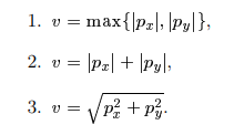
If p_x, p_y were grey values produced by applying P_x, P_y to an img, the output grey value v can be chosen by :
Example
(1) Read img
> ic=imread('ic.tif');
(2) Applying each of P_x and P_y individually
- P_x for Vertical edge, P_y for Horizontal edge
# (a) Vertical edge detection
>> px=[-1 0 1;-1 0 1;-1 0 1];
>> icx=filter2(px,ic);
>> figure,imshow(icx/255)

# (b) Horizontal edge detection
>> py=px’;
>> icy=filter2(py,ic);
>> figure,imshow(icy/255)
(3) Contain all the edges by any of upper 3 methods
# (a) All edges detection
>> edge_p=sqrt(icx.^2+icy.^2);
>> figure,imshow(edge_p/255)

# (b) Binary img containing edges by thresholding
>> edge_t=im2bw(edge_p/255,0.3);
(4) Prewitt filters by *edge function
*edge function
: taking care of all the filtering & choosing a suitable threshold level & extra processing
- Detected edges can be changed by specifying a threshold level
>> edge_p=edge(ic,'prewitt');
>> figure,imshow(edge_p)
Roberts cross-gradient filters

>> edge_r=edge(ic,'roberts');
>> figure,imshow(edge_r)
Sobel filters
- similar to Prewitt filters : smoothing filter in the opposite direction to the central difference filter
- [1 2 1] : slightly more prominence to the central pixel than Prewitt filters
- The best edge detection filter & performing well in the presence of noise

>> edge_s=edge(ic,'sobel');
>> figure,imshow(edge_s)
8.3 Second differences
8.3.1 The Laplacian
1) Edge-detection by Second difference (=Difference of differences)
To calculate a (central) second difference, take the Backward difference of a Forward difference
→ Sum of two second differences is implemented by Discrete Laplacian filter


2) How the second difference affects an edge
(b) A ramp edge function
[8.4] Difference of the edge function
[8.10] Second differences of the edge function


3) MATLAB function fspecial
- ALPHA : optional parmameter (default=0.2)
>> l=fspecial('laplacian', ALPHA);
Laplacian (after taking an absolute value, or squaring)
- Disadvantage : Double edges → Sensitive to noise (messy than Prewitt or Sobel methods)
- Advantage : Detecting edges in all directions equally well

>> l=fspecial('laplacian',0);
>> ic_l=filter2(l,ic);
>> figure,imshow(mat2gray(ic_l))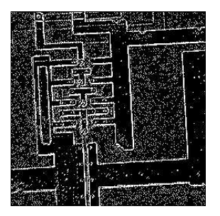
Other Laplacian masks

8.3.2 Zero crossings
1) Laplace filtering
: To find the position of edges by locating zero crossings
The position of the edge
= The place where the value of the filter takes on a zero value after Laplace filtering
= The place where the result of the filter changes sign

2) Zero crossings
(1) Define the zero crossings
in such a filtered img to be pixels which satisfy either of the following :
1. they have a negative grey value and are next to (by four-adjacency) a pixel whose grey value is positive,
2. they have a value of zero, and are bw negative and positive valued pixels
Circle-shape zero-crossing : across any edge there can be only one zero-crossing
→ So, img formed from zero-crossings has the potential to be very neat(정돈 된)
(2) zerocross option of edge function
: taking the zero crossings after filtering with a given filter (ex. laplace, log)
◾ Example of not a good method
- Applying Laplace filter directly and Finding its Zero crossings
- Result : too many grey level changes have been interpreted as edges
>> l=fspecial('laplace',0);
>> icz=edge(ic,'zerocross',l);
>> imshow(icz)
◾ Marr-Hildreth method
- Applying LoG filter and Finding its Zero crossings BY
① Smooth the image with a Gaussian filter
② Convolve the result with a Laplacian
③ Find the Zero crossings
- Result : edge detected as close as possible to biological vision
① + ② = 'log' option (LoG, Laplacian of Gaussian) for fspecial function
③ 'zerocross' option for edge function
>> log=fspecial('log',13,2);
>> mh=edge(ic,'zerocross',log);
>> imshow(mh)
8.4 Edge Enhancement
1) Unsharp masking
(1) Unsharp masking
- How : Subtracting a scaled blurred img from the original
- Result : the edges are cisper and more clearly defined (b) = Edge Enhancement

>> f=fspecial('average'); # Blur
>> xf=filter2(f,x);
>> xu=double(x)-xf/1.5 # Scale and Subtract
>> imshow(xu/70) # Scale for display
(2) Implementation

- Considering the function of grey values as we travel across on edge
- Performing the blur filtering and subtracting operation in one command using linearity of the filter
Unsharp masking can be implemented by a filter of the form :

(3) 'unsharp' option of fspecial function
- α : an optional parameter (default=0.2)

- ex. α=0.5 the filter is

>> p=imread('pelicans.tif');
>> u=fspecial('unsharp',0.5);
>> pu=filter2(u,p);
>> imshow(p),figure,imshow(pu/255)
2) High boost filtering
(1) High boost filters

A : amplification factor ( If A=1, high boost filter = ordinary high pass filter )
>> f=[-1 -1 -1;-1 11 -1;-1 -1 -1]/9;
>> xf=filter2(x,f);
>> imshow(xf/80)
(2) How to obtain the best results for high boost filtering
Multiply the equation by a factor w so that the filter values sum to 1 ; this requires

(3) General unsharp masking formula

(+) Example

(4) Implementation of high boost filters
By using the identity and averaging filters
>> id=[0 0 0;0 1 0;0 0 0];
>> f=fspecial('average');

>> hb1=3*id-2*f
hb1 =
    -0.2222  -0.2222  -0.2222
    -0.2222   2.7778  -0.2222
    -0.2222  -0.2222  -0.2222

>> hb2=1.25*id-0.25*f
hb2 =
    -0.0278  -0.0278  -0.0278
    -0.0278   1.2222  -0.0278
    -0.0278  -0.0278  -0.0278


>> x1=filter2(hb1,x);
>> imshow(x1/255)
8.5 Final Remarks
There are many different edge detection algorithms
- Implemented in the 'edge' function of the MATLAB image Processing Toolbox / MATLAB programs
- Highly subjective → The choice of an suitable edge detector will depend on the nature of img, the amount (and type) of noise, and the use for which the edges are to be put
'DIP > Matlab' 카테고리의 다른 글
| [Ch10] The Hough and Distance Transform (0) | 2023.01.09 |
|---|---|
| [Ch9] The Fourier Transform (0) | 2022.03.06 |
| [Ch7] Noise (0) | 2022.02.12 |
| [Ch6] Spatial Filtering (0) | 2022.02.08 |
| [Ch5] Pointing Processing (0) | 2022.02.07 |