
티스토리 뷰
9.1 Introduction
Fourier Transform
- A powerful alternative to linear spatial filtering ; more efficient than using a spatial filter for a large filter
- Isolating and processing particular img 'frequencies' → Performing low/high-pass filtering with a great precision
9.2 The one-dimensional Discrete Fourier Transform
1) Approximation of the periodic function
(1) Periodic function
- Written as the sum of (= its decomposition into) sine or cosine functions of varying amplitudes and frequencies
(2) Approximation of the original function
- Required a finite (or an infinite) number of functions in their decomposition
- The more terms of the series, the closer the sum will approach the original function
- FT to obtain individual sine waves which compose a given function or sequence
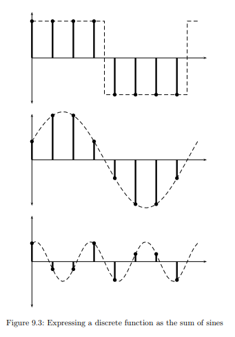
- Ex. A square wave and its approximation

(3) Discrete Approximation of the original function for img
- Only need a finite number of functions to obtain a finite number of values
- DFT to obtain individual sine waves which compose a given discrete function or sequence
- Ex. Discrete approximation to the square wave => the sum of only 2 sine functions

2) Definition of the one dimensional DFT
(1) The supposed sequence of length N

(2) The formula for the (forward) DFT

3) The Inverse DFT
(1) The formula for the Inverse DFT

(2) Comparison with forward transform (DFT)

4) Implementation in MATLAB
(1) The forward DFT : fft (Fast Fourier Transform, which is a fast and efficient method for DFT)
(2) The inverse DFT : ifft
※ To apply a DFT to a single vector, use a column vector !
a =
	1 2 3 4 5 6


>> fft(a’)

ans =
    21.0000
    -3.0000 + 5.1962i
    -3.0000 + 1.7321i
    -3.0000
    -3.0000 - 1.7321i
    -3.0000 - 5.1962i
9.3 Properties of the one-dimensional DFT
1) Linearity
- f and g : two vectors of equal length
- p and q : scalars
- F, G and H : DFT's of f, g and h
∴ h = pf + qg → H = pF + qG
2) Shifting
- Multiply each element x_n of a vector x by (-1)^n to change the sign of every seconed element
- Resulting vector : x'
∴ The DFT X' of x' = The DFT X of x with swapping of the left and right halves
>>  x = [2 3 4 5 6 7 8 1];

>>  x1=(-1).^[0:7].*x

x1 =
     2    -3     4    -5     6    -7     8    -1


>> X=fft(x')

X =
  36.0000 + 0.0000i
  -9.6569 + 4.0000i
  -4.0000 - 4.0000i
   1.6569 - 4.0000i
   4.0000 + 0.0000i
   1.6569 + 4.0000i
  -4.0000 + 4.0000i
  -9.6569 - 4.0000i


>> X1=fft(x1')

X1 =
   4.0000 + 0.0000i
   1.6569 + 4.0000i
  -4.0000 + 4.0000i
  -9.6569 - 4.0000i
  36.0000 + 0.0000i
  -9.6569 + 4.0000i
  -4.0000 - 4.0000i
   1.6569 - 4.0000i
The first four elements of X = The last four elements of X1, and vice versa
3) Conjugate symmetry

4) The Fast Fourier Transform
(1) FFT
: extremly fast and efficient algorithms for computing a DFT
- To reduce the time needed to compute a DFT
- One FFT method works recursively by..
dividing the original vector into two halves, computing the FFT of each half, and then putting the results together
- most efficient when the vector length = 2^n (the power of 2)
(2) Direct arithmetic VS FFT
The number of multiplications required for each method for a vector of length 2^n
- Direct arithmetic : (2^n)^2 = 2^(2n) multiplications
- FFT : n*2^n
∴ The saving in time = an order of 2^n/n : the advantages of FFT increases as the size of the vector increases

9.4 The two-dimensional DFT
Some properties of the two dimensional DFT
9.5 Fourier Transforms in MATLAB
9.6 Fourier Transforms of images
9.7 Filtering in the frequency domain
9.8 Removal of periodic noise
9.9 Inverse fitering
'DIP > Matlab' 카테고리의 다른 글
| [Ch11] Morphology (0) | 2023.01.09 |
|---|---|
| [Ch10] The Hough and Distance Transform (0) | 2023.01.09 |
| [Ch8] Edges (0) | 2022.02.20 |
| [Ch7] Noise (0) | 2022.02.12 |
| [Ch6] Spatial Filtering (0) | 2022.02.08 |