티스토리 뷰
1) 확률분포 : 확률 변수가 특정한 값을 가질 확률을 나타내는 함수
(1) 이산확률분포 : 확률변수 X의 개수를 정확히 셀 수 있을 때 (Discrete 값)
(2) 연속확률분포 : 확률변수 X의 개수를 정확히 셀 수 없을 때 (Continuous 값)
- 확률밀도함수로 표현 (Ex) 정규분포(Normal distribution)
- 실제 세계의 많은 데이터는 정규분포로 표현 가능
2) 이미지 데이터에 대한 확률분포
: 이미지에서의 다양한 특징들이 각각의 확률 변수가 되는 분포 (다변수 확률분포)
- 이미지 데이터는 다차원 특징 공간의 한 점으로 표현됨 → 이미지의 분포를 근사하는 모델 학습 가능
- 사람 얼굴에는 통계적인 평균치가 존재 → 모델은 이를 수치적으로 표현 가능
9.1 AE 소개 및 학습 원리
1) 정의

AutoEncoder : 데이터에 대한 효율적인 압축을 신경망을 통해 자동으로 학습하는 모델
Ex) AE, VAE(Variational AE), DAE(Denoising AE), SAE, SDAE, CAE, SCAE
2) 주요기능 및 특징
(1) 주요 기능
1) Dimension Reduction (차원 축소)
2) Density Estimation (확률분포 예측)
(2) 특징
◾ Unsupervised learning
: 입력 데이터 자체가 라벨로 사용되는 비지도 학습
◾ Manifold learning (Encoder)
= Efficient data coding
= Feature learning
= Representation learning
= (Nonlinear) Dimensionality reduction
: 입력 데이터의 차원보다 낮은 차원으로 압축
https://jeonggg119.tistory.com/30?category=1052481
[Ch2] Manifold Learning
[Keyword] : Manifold Learning, Unsupervised Learning 1. AutoEncoder의 주요 기능 1) Dimension Reduction (차원 축소) : Unsupervised Learning Task 2) Density Estimation (확률 분포 예측) 3) 'Manifold'..
jeonggg119.tistory.com
◾ Generative model learning (Decoder)
◾ Maximum Likelihood density Estimation (MLE)
: 주어진 데이터만을 토대로 가정된 확률분포의 parameter를 추정하는 방법 (원하는 정답이 나올 확률을 최대로 만들도록)
→ AE DNN 학습하는 것 = MLE 관점에서의 최적화
Loss function viewpoints 2 : Maximum likelihood
1) 핵심
Network의 출력값 p( y | f(x) ) = 우리가 정해놓은 확률분포 모델의 Parameter (Likelihood 값이 X)
2) Define functions
Conditional probability 확률분포 모델을 추가로 정하고 시작 (Ex. Gaussian, Bernoulli)
모델의 Parameter를 추정하는 것 (Ex. Gaussian 모델이면 평균이랑 표준편차)
3) Learning (Training)
(1) Model Output
Network의 출력값(확률분포 모델의 평균값)이 Given 일 때,
원하는 정답 y가 나올 확률을 최대로 하고 싶음
= 확률분포에 대한 Maximum Likelihood (확률) 값 찾고 싶음
← When? 확률분포 모델의 평균값 = 정답 y값
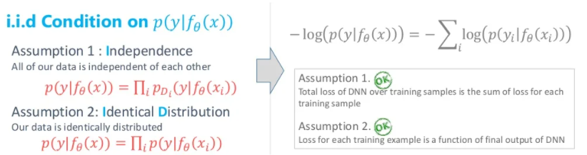
(2) Loss : - log p
iid Condition 성립함
(3) 장점
확률분포 모델을 찾은 것이므로 Sampling 가능
고정 입력 → 고정 / 다른 출력

AutoEncoder를 학습할 때
- 학습방법은 Unsupervised learning
- Loss는 negative MLE
학습된 AutoEncoder 에서
- Encoder는 차원 축소 (Manifold learning)
- Decoder는 생성 모델 (Generative model)
3) 모델 구조


입력 x가 들어와 신경망(Encoder)을 통과해 가장 압축된 잠재 변수(Latent variable) z가 됨
압축된 z는 다시 신경망(Decoder)을 통과해 복원되어 출력 y가 됨 (=Reconstruct Input)
(1) x, y ∈ R^d : Input layer 와 Output layer의 size 같음 (같은 Dimension) → z : Dimension 축소됨
(2) Loss L(x, y) encourages Output to be close to Input : 입출력이 동일한 Network
(3) 학습이 끝나면 Encoder와 Decoder를 따로 떼어 사용함
- Encoder : 최소한 학습 데이터는 잘 압축해서 latent vector로 표현할 수 있게 됨 → 데이터 추상화에 많이 사용
입력 샘플을 잠재 공간, 즉 인코더에 의해 정의된 숨겨진 구조화된 값 집합에 매핑하는 함수 (압축)
- Decoder : 최소한 학습 데이터는 생성해낼 수 있게 됨 → but, 생성된 데이터가 학습 데이터를 좀 닮아 있음
이 잠재 공간의 요소를 사전 정의된 타겟 도메인으로 매핑하는 여함수 (복원)
cf) GAN : AutoEncoder와 달리 Minimum 성능보장이 없어서 학습이 좀 어려움
4) Train
AE의 목적 : 압축
→ 입력값 x 자체를 목표(라벨)값으로 설정
→ 출력값 x' 과 입력값 x 간의 차이로 Loss 계산
Ex) L(x, x') = ∑ | x - x' | : x와 x'에서 같은 위치에 있는 픽셀 간의 절댓값 차이를 다 더한 L1 Loss
# ANN으로 만든 AE (+ Activation function 생락)
class Autoencoder(nn.Module):
    def __init__(self):
        super(Autoencoder,self).__init__()
        self.encoder = nn.Linear(28*28,20) # 데이터를 길이 20 벡터로 압축
        self.decoder = nn.Linear(20,28*28) # 압축된 벡터를 원 크기로 복원

    def forward(self,x):
        x = x.view(batch_size,-1) # [B,1,28,28] -> [B,784]
        encoded = self.encoder(x)
        out = self.decoder(encoded).view(batch_size,1,28,28)
        return out


# Loss function & Optimizer
device = torch.device("cuda:0" if torch.cuda.is_available() else "cpu")
model = Autoencoder().to(device)
loss_func = nn.MSELoss()
optimizer = torch.optim.Adam(model.parameters(), lr=learning_rate)

# Train
loss_arr =[]
for i in range(num_epoch):
    for j,[image,label] in enumerate(train_loader):
        x = image.to(device)

        optimizer.zero_grad()
        output = model.forward(x)
        loss = loss_func(output,x)
        loss.backward()
        optimizer.step()

    if j % 1000 == 0:
        print(loss)
        loss_arr.append(loss.cpu().data.numpy()[0])

# Check with train image
out_img = torch.squeeze(output.cpu().data)
print(out_img.size())
for i in range(10):
    plt.imshow(torch.squeeze(image[i]).numpy(),cmap='gray')
    plt.show()
    plt.imshow(out_img[i].numpy(),cmap='gray')
    plt.show()
5) Test
with torch.no_grad():
  for i in range(1):
      for j,[image,label] in enumerate(test_loader):
          x = image.to(device)

          optimizer.zero_grad()
          output = model.forward(x)

      if j % 1000 == 0:
          print(loss)


out_img = torch.squeeze(output.cpu().data)
print(out_img.size())

for i in range(10):
    plt.imshow(torch.squeeze(image[i]).numpy(),cmap='gray')
    plt.show()
    plt.imshow(out_img[i].numpy(),cmap='gray')
    plt.show()
9.2 Convolutional AE
1) Transposed convolution
(1) Encoder VS Decoder
- 압축하는 Encoder 부분 : Classification model에서 Feature extract 하는 부분을 사용
- 복원하는 Decoder 부분 : Encoder와 대칭되게 만들고자 Transposed convolution (Deconvolution) 사용
(2) Convolution VS Transposed Conv : 가중치가 입력과 곱해지는 방식의 차이
- Convolution : 입력값에 필터의 가중치를 각각 곱한 결과의 합
- Transposed Conv : 하나의 입력값을 받아 서로 다른 가중치들을 곱해 '필터의 크기만큼' 퍼뜨림
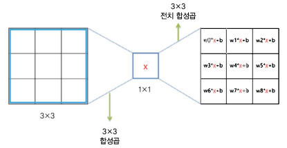
(3) Transposed Conv 원리
torch.nn.ConvTranspose2d(in_channels, out_channels, kernel_size, stride=1, padding=0,
						 output_padding=0, groups=1, bias=True, dilation=1)
- Conv 에서 padding : 입력값 둘레에 값을 추가하는 역할
- Transposed Conv 에서 padding : 결괏값에서 제일 바깥 둘레를 빼주는 역할
- Transposed Conv 에서 output_padding : 결과로 나오는 텐서의 크기를 맞추고자 padding으로 잘리는 부분을 줄이는 역할
- padding 없이 output_padding 만 주면 padding으로 줄어든 부분이 없으므로 테두리가 0으로 채워지는 결과


(4) Transposed Conv 체커보드 아티팩트 한계점 해결 : Resize Convolution
보통 입력 이미지에서 특성을 뽑아내고 크기를 줄일 때 1/2로 많이 줄이기에,
Transposed Conv를 할 때도 결과 텐서의 가로 세로가 입력의 2배가 되도록 설정함
Transposed Conv에서 stride = 2 이상을 사용하면 겹치는 부분 때문에 체커보드 아티팩트 문제 발생
→ 해결하고자 Transposed Conv 대신 Bilinear이나 Nearest Neighbor 등의 Upsampling 연산을 낮은 해상도 이미지에 먼저 적용한 후, stride = 1 Conv 연산을 적용해 아티팩트 줄임
2) 모델 구조
(1) 압축하는 Encoder 부분 : Classification model에서 Feature extract 하는 부분을 사용
" 몇 번의 Convolution 연산 이후에 2x2 Max pooling으로 Feature map size 감소 "
→ Encoder 통과하면 압축 가능
class Encoder(nn.Module):
    def __init__(self):
        super(Encoder,self).__init__()
        self.layer1 = nn.Sequential(
                        nn.Conv2d(1,16,3,padding=1),                            # batch x 16 x 28 x 28
                        nn.ReLU(),
                        nn.BatchNorm2d(16),
                        nn.Conv2d(16,32,3,padding=1),                           # batch x 32 x 28 x 28
                        nn.ReLU(),
                        nn.BatchNorm2d(32),
                        nn.Conv2d(32,64,3,padding=1),                           # batch x 32 x 28 x 28
                        nn.ReLU(),
                        nn.BatchNorm2d(64),
                        nn.MaxPool2d(2,2)                                       # batch x 64 x 14 x 14
        )
        self.layer2 = nn.Sequential(
                        nn.Conv2d(64,128,3,padding=1),                          # batch x 64 x 14 x 14
                        nn.ReLU(),
                        nn.BatchNorm2d(128),
                        nn.MaxPool2d(2,2),
                        nn.Conv2d(128,256,3,padding=1),                         # batch x 64 x 7 x 7
                        nn.ReLU()
        )


    def forward(self,x):
        out = self.layer1(x)
        out = self.layer2(out)
        out = out.view(batch_size, -1)
        return out
(2) 복원하는 Decoder 부분 : Encoder와 대칭되게 만들고자 Transposed convolution (Deconvolution) 사용
" kernel_size=3, stride=2, padding=1, output_padding=1 로 하면 Feature map size가 2배로 늘어남 "
→ Decoder 통과하면 원래 데이터 크기로 돌아가도록 만들 수 있음 (복원)
class Decoder(nn.Module):
    def __init__(self):
        super(Decoder,self).__init__()
        self.layer1 = nn.Sequential(
                        nn.ConvTranspose2d(256,128,3,2,1,1),                    # batch x 128 x 14 x 14
                        nn.ReLU(),
                        nn.BatchNorm2d(128),
                        nn.ConvTranspose2d(128,64,3,1,1),                       # batch x 64 x 14 x 14
                        nn.ReLU(),
                        nn.BatchNorm2d(64)
        )
        self.layer2 = nn.Sequential(
                        nn.ConvTranspose2d(64,16,3,1,1),                        # batch x 16 x 14 x 14
                        nn.ReLU(),
                        nn.BatchNorm2d(16),
                        nn.ConvTranspose2d(16,1,3,2,1,1),                       # batch x 1 x 28 x 28
                        nn.ReLU()
        )

    def forward(self,x):
        out = x.view(batch_size,256,7,7)
        out = self.layer1(out)
        out = self.layer2(out)
        return out
3) Train
device = torch.device("cuda:0" if torch.cuda.is_available() else "cpu")

encoder = Encoder().to(device)
decoder = Decoder().to(device)

# 인코더와 디코더의 파라미터를 동시에 학습시키고자 묶음
parameters = list(encoder.parameters())+ list(decoder.parameters())

loss_func = nn.MSELoss()
optimizer = torch.optim.Adam(parameters, lr=learning_rate)


try:
    encoder, decoder = torch.load('./model/conv_autoencoder.pkl') # 모델 load
    print("\n--------model restored--------\n")
except:
    print("\n--------model not restored--------\n")
    pass

# Train
for i in range(num_epoch):
    for j,[image,label] in enumerate(train_loader):
        optimizer.zero_grad()
        image = image.to(device)

        output = encoder(image)
        output = decoder(output)

        loss = loss_func(output,image)
        loss.backward()
        optimizer.step()

    if j % 10 == 0:
        torch.save([encoder,decoder],'./model/conv_autoencoder.pkl') # 모델 저장
        print(loss)

# Check with Train image
out_img = torch.squeeze(output.cpu().data)
print(out_img.size())

for i in range(5):
    plt.subplot(1,2,1)
    plt.imshow(torch.squeeze(image[i]).cpu().numpy(),cmap='gray')
    plt.subplot(1,2,2)
    plt.imshow(out_img[i].numpy(),cmap='gray')
    plt.show()
4) Test
with torch.no_grad():
    for j,[image,label] in enumerate(test_loader):

        image = image.to(device)
        output = encoder(image)
        output = decoder(output)

    if j % 10 == 0:
        print(loss)

out_img = torch.squeeze(output.cpu().data)
print(out_img.size())

for i in range(5):
    plt.subplot(1,2,1)
    plt.imshow(torch.squeeze(image[i]).cpu().numpy(),cmap='gray')
    plt.subplot(1,2,2)
    plt.imshow(out_img[i].numpy(),cmap='gray')
    plt.show()
DAE (Denoisng AE)
noise = init.normal_(torch.FloatTensor(batch_size,1,28,28),0,0.1)
noise_image = image + noise
1) DAE 구조
(1) DAE : AE의 입력 x에 Noise (Stochastic perturbation) 추가한 것
- Encoder의 입력 : ~x = x + Noise q
- Decoder의 출력 : y = x (Noise 추가되기 전 입력과 같도록 학습)
(2) Noise 포함된 입력을 넣어 Reconstruction하면 Denoised 된 결과 나옴
사람이 같은 의미를 갖는 샘플이라고 생각할 수 있는 수준의 Noise를 추가함


2) Evalutation (Performace)
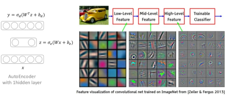
(1) Visualization of learned filters
Filters in 1 hidden layer architecture must capture low-level features (Edge 성분) of images
랜덤값으로 초기화하였기에 노이즈처럼 보이는 필터일수록 학습이 잘 안된 것, Edge filter 모습일수록 잘 된 것


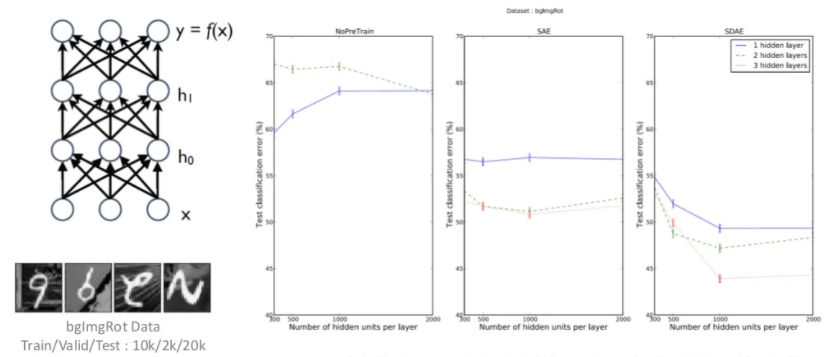
(2) SDAE : Pretraining

(3) Generation
- 각 layer별 출력값을 Bernoulli 확률값으로 해석하면, 확률분포모델이 정해지기에 Sampling이 가능
- Sampling 다양하게 해서 비슷한 여러 이미지 생성할 수 있음

3) SCAE (Stochastic Contractive AutoEncoder)
(1) DAE에서 입력에 Noise 추가했던 목적
: 의미적으로 같지만 (Manifold 상에서 같은 위치에 mapping) 원래 데이터 공간에서 다른 것들을 만들기 위해 추가
(2) SCAE
: 입력에 Noise를 추가하는 것 대신 Regularization term을 통해 Manifold 상에서 같은 위치로 mapping 하는 것 구현

VAE (Variational AE)
: Latent variable이 어떻게 분포하는지, 어떤 값이 바뀌면 결과가 얼마나 바뀌는지 등을 알아내고자
Latent variable 공간을 친숙한 정규분포 공간으로 맞춰주는 방법
AE와 VAE는 목적 자체가 정반대
- AE : 앞단(Encoder 부분) 학습 위해 뒷단 추가 → Manifold learning
- VAE : 뒷단(Decoder 부분) 학습 위해 앞단 추가 → Generative model learning
[Ch4] Variational AutoEncoders (VAE, CVAE, AAE)
AE와 VAE는 목적 자체가 정반대 - AE : 앞단(Encoder 부분) 학습 위해 뒷단 추가 → Manifold learning - VAE : 뒷단(Decoder 부분) 학습 위해 앞단 추가 → Generative model learning [Keyword] : Generative..
jeonggg119.tistory.com
9.3 Semantic Segmentation
1) U-Net
: 의료(생체) 데이터 이미지에서 Segmentation 작업을 수행하기 위해 만들어진 모델


2) 입출력 형태 및 손실함수
Ex1) 세포 단면 흑백 이미지에서 세포 간 경계선을 구분하는 Binary Segmentation Task
- 입력 : 채널이 1개인 흑백 이미지
- 결과 : 채널이 2개인 Tensor (각 채널은 해당 픽셀이 세포의 경계선에 해당하는지, 아닌지에 대한 수치)
→ 첫 번째 채널의 수치가 더 크면 세포의 경계선, 두 번째 채널의 수치가 더 크면 세포의 내부
- 손실함수 : BCE Loss
Ex2) 컬러 이미지에서 k개의 클래스로 구분되는 Multi-class Segmentation Task
- 입력 : 채널이 3개인 컬러 이미지
- 결과 : 채널이 k개인 Tensor
- 손실함수 : CE Loss
3) 모델 구조
전체적으로 Convolutional AutoEncoder의 형태 + Skip-connection (Copy and crop 연산)
Skip-connection : [ResNet] Tensor 간의 합 / [U-net] Tensor 간의 채널 Concatenation
AE에서는 입력 이미지가 압축되는 과정에서 위치정보의 손실 발생
→ 다시 원본 크기로 복원하는 과정에서 정보 부족해 원래 위치에서 이동(차이) 발생
복원 과정에 Skip-connection 사용하면 원본 이미지의 위치 정보를 추가적 전달받을 수 있음 !
→ 비교적 정확한 위치 복원 가능 + 더 좋은 Segmentation 결과
4) 코드 구현
def conv_block(in_dim,out_dim,act_fn):
    model = nn.Sequential(
        nn.Conv2d(in_dim,out_dim, kernel_size=3, stride=1, padding=1),
        nn.BatchNorm2d(out_dim),
        act_fn,
    )
    return model

def conv_trans_block(in_dim,out_dim,act_fn):
    model = nn.Sequential(
        nn.ConvTranspose2d(in_dim,out_dim, kernel_size=3, stride=2, padding=1,output_padding=1),
        nn.BatchNorm2d(out_dim),
        act_fn,
    )
    return model

def maxpool():
    pool = nn.MaxPool2d(kernel_size=2, stride=2, padding=0)
    return pool

def conv_block_2(in_dim,out_dim,act_fn):
    model = nn.Sequential(
        conv_block(in_dim,out_dim,act_fn),
        nn.Conv2d(out_dim,out_dim, kernel_size=3, stride=1, padding=1),
        nn.BatchNorm2d(out_dim),
    )
    return model


class UnetGenerator(nn.Module):
    def __init__(self,in_dim,out_dim,num_filter):
        super(UnetGenerator,self).__init__()
        self.in_dim = in_dim
        self.out_dim = out_dim
        self.num_filter = num_filter
        act_fn = nn.LeakyReLU(0.2, inplace=True)

        print("\n------Initiating U-Net------\n")

        self.down_1 = conv_block_2(self.in_dim,self.num_filter,act_fn)
        self.pool_1 = maxpool()
        self.down_2 = conv_block_2(self.num_filter*1,self.num_filter*2,act_fn)
        self.pool_2 = maxpool()
        self.down_3 = conv_block_2(self.num_filter*2,self.num_filter*4,act_fn)
        self.pool_3 = maxpool()
        self.down_4 = conv_block_2(self.num_filter*4,self.num_filter*8,act_fn)
        self.pool_4 = maxpool()

        self.bridge = conv_block_2(self.num_filter*8,self.num_filter*16,act_fn)

        self.trans_1 = conv_trans_block(self.num_filter*16,self.num_filter*8,act_fn)
        self.up_1 = conv_block_2(self.num_filter*16,self.num_filter*8,act_fn)
        self.trans_2 = conv_trans_block(self.num_filter*8,self.num_filter*4,act_fn)
        self.up_2 = conv_block_2(self.num_filter*8,self.num_filter*4,act_fn)
        self.trans_3 = conv_trans_block(self.num_filter*4,self.num_filter*2,act_fn)
        self.up_3 = conv_block_2(self.num_filter*4,self.num_filter*2,act_fn)
        self.trans_4 = conv_trans_block(self.num_filter*2,self.num_filter*1,act_fn)
        self.up_4 = conv_block_2(self.num_filter*2,self.num_filter*1,act_fn)

        self.out = nn.Sequential(
            nn.Conv2d(self.num_filter,self.out_dim,3,1,1),
            nn.Tanh(),  #필수는 아님
        )

    def forward(self,input):
        down_1 = self.down_1(input)
        pool_1 = self.pool_1(down_1)
        down_2 = self.down_2(pool_1)
        pool_2 = self.pool_2(down_2)
        down_3 = self.down_3(pool_2)
        pool_3 = self.pool_3(down_3)
        down_4 = self.down_4(pool_3)
        pool_4 = self.pool_4(down_4)

        bridge = self.bridge(pool_4)

        trans_1 = self.trans_1(bridge)
        concat_1 = torch.cat([trans_1,down_4],dim=1)
        up_1 = self.up_1(concat_1)
        trans_2 = self.trans_2(up_1)
        concat_2 = torch.cat([trans_2,down_3],dim=1)
        up_2 = self.up_2(concat_2)
        trans_3 = self.trans_3(up_2)
        concat_3 = torch.cat([trans_3,down_2],dim=1)
        up_3 = self.up_3(concat_3)
        trans_4 = self.trans_4(up_3)
        concat_4 = torch.cat([trans_4,down_1],dim=1)
        up_4 = self.up_4(concat_4)
        out = self.out(up_4)
        return out
batch_size = 16
img_size = 256
in_dim = 1
out_dim = 3
num_filters = 16
sample_input = torch.ones(size=(batch_size,1,img_size,img_size))
model = UnetGenerator(in_dim=in_dim,out_dim=out_dim,num_filter=num_filters)
output = model(sample_input)
print(output.size())
'DL > Pytorch' 카테고리의 다른 글
| [Ch10] 생성적 적대 신경망(GAN) (0) | 2022.02.02 |
|---|---|
| [Ch8] Neural Style Transfer (0) | 2022.01.24 |
| [Ch7] 학습 시 생길 수 있는 문제점 및 해결방안 (0) | 2022.01.22 |
| [Ch6] 순환신경망(RNN) (0) | 2022.01.20 |
| [Ch5] 합성곱 신경망(CNN) (0) | 2022.01.15 |